Determining the Base Note of a Musical Scale

When a musical sequence of notes is played, there is a mental requirement of sorts that it must end on a certain note or it will seem incomplete.  For example, if you play the white keys on a piano from middle C up to B and then stop, it will seem ‘not right’, and part of your brain will almost be begging you to play that final C above middle C.  The same is true if we were to play all those keys in a random order – our stopping place would need to end on a C (any C on the keyboard) or it would feel like the wrong place to end.

When a different selection of notes is used the required end note may change.  For example, with the selection of notes C,D,F,G,A – the end note changes to F.  And for C,D,G,A – G makes a good ending, although C is still acceptable.

The collection of white notes from C to B describes the well-known scale of C-Major and pieces written in it almost always end with a C.  But the requirement is not rigid.  There is a degree of suitability to how acceptable a note will be to end with.  In C-major the note E also sounds quite reasonable to end with; note G: less so; note A: less again; and note B: definitely not!

We can refer to the ending note as the base note because it is what a musical scale is based around.  Given a set of notes then, what determines which will be base?  The answer is by no means simple.  To begin with we need to determine how to compare just two notes.

Comparing two notes

While it is rare for music to be written using only two notes, it is still possible to compare them to determine which is base with careful listening.  Doing so requires a digital instrument because acoustic ones will always be slightly out of tune and, as will be seen, the requirements for frequency accuracy are very precise.  The following method will be used:

We arrive up at the following table, where ‘Note’ refers to the note above middle C and ‘Base’ refers to which of them (C or the higher note) is base.

Note	Base
C#	C#
D	C
D#	C
E	C
F	F
F#	neither
G	C
G#	G#
A	A
A#	A#
B	C

(Table 1)

This shows which note is base when compared with C.  For D, D#, and E, C is base.  But for C# and F, they are base.

For F# is says ‘neither’ because C and F# are equidistant and neither can be preferred.  To explain, suppose you listened to C and F# and concluded C was base.  But because of ‘transposition’, we can move F# down an octave and should get the same result; which means we now are comparing the F# below middle C with C.  But we can now add 6 semitones to each of these notes, transposing them upward, and F# becomes middle C and C becomes F#.  This makes the old base note now the F#, which contradicts what you believed earlier.

A second important point is that the upper octave from G to B will be the inverse of the lower octave from D# to F.  For example, if we compare C and G, we can transpose G to the G below middle C.  We then add 5 semitones to each and the G becomes C and the old C becomes F.  Thus C-G is the opposite of C-F, and since F is base for C-F, C must be base for C-G.  So we only need to study the lower octave between C and F# to know the upper octave.

For C and C#, it might be difficult to determine which is base.  This happens when two notes are close together.  So instead we’ll compare the C-B combination and take the inverse of it.  You can still compare C and C#, it just requires more careful listening.

A final point is we tend to have a bias toward picking the lower frequency note as base.  This might cause you to decide that C is the base of C-F.  To get around this problem, transpose the upper note down an octave.  In this case, you will be comparing F below C with C, which will make the F stand out as the obvious base.  Once you are aware of this bias it should be easy to adjust for it without transposing.

Numbering the notes

Let’s start referring to the notes using numbers.  We’ll refer to middle C as 0 (zero).  Each higher number will represent a semitone spacing.  So 1 will be C#, 2 will be D, 6 will be F#, -1 will be the B below middle C, etc.  This is a useful scale because it overlays the 12-tone equal-temperament (a.k.a. Western) scale and also allows us to refer to notes in-between the semitones, which we will be doing a lot of.

Next let’s introduce the concept of energy.  Musical pieces tend to end by ‘fading out’, which they do by reducing in loudness/volume, reducing rhythm speed, and often end on a low-frequency note.  All of these things are a reduction in measurable sound energy.  So it seems appropriate to describe the base note as also being the note of lower energy, even though it may be of higher frequency, which has higher sound energy.

Using this numbering system and energy concept we can convert the above table into a chart.  To do this, the note numbers will be on the x-axis and the y-axis will represent energy.  When the comparison note is not the base it will have a value of 1, and when note 0 is base, the comparison note will have a value of -1.  In this way the base note will always have the lower energy.  This gives the chart:

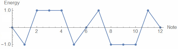
(Chart 1)

The chart goes from 0 to 12, i.e. middle C to the C above it.  It is zero at both C’s and at note 6 (F#).  We can also see the upper half octave is a double mirror image of the lower half octave (mirrored on x-axis and around note 6), which is due to the transposing described earlier.

Looking at the lower half-octave, it appears that the middle section favours C (note 0) as base and the outer notes favour themselves as base.  Is that how it works?  No, not at all.  In fact the relationship is far more complex and this chart barley reveals anything.  There is a lot happening between those semitones.

Memory buffers

The audio processing part of our brain appears to have a short-term memory buffer that accurately remembers frequency information of around the past 7 seconds.  With this it is able to compare them and determine which are relatively base.  Careful experimenting suggests the exact duration is close to 7.144 seconds.

Once this interval has passed, the information then appears to transfer to a secondary buffer of the same duration.  With this it makes additional but different comparisons with the frequencies in the first buffer.

Beyond this are three additional buffers of the same duration.  They are used for processing a special nullification process.  Finally, there are two additional accurate long-term memory buffers located approximately between 2:50 and 8:30, which will be discussed later.

Interactive Apps

A number of interactive applications are provided to assist with demonstrating what’s described.  Here is the first one:

Compare Frequencies    (opens in new tab)

This allows frequencies to be compared.  Note values can be entered and played as perfect sine waves.  Much of the experimenting involves alternating between note 0 and another note to hear which is base.  This can be done by entering ‘0’ in the first field and the other note value in the field below it, then pressing, back-and-forth, the keyboard keys A and S, then stopping on one to hear if it is base.

This app also shows the first four memory buffers.  This will be useful for much of the testing here.  In general, wait for the primary and secondary buffers to become empty before starting a new test.

Here’s another:

Sine Wave Piano    (opens in new tab)

This allows frequencies to be played using a piano keyboard as input.  It works only with whole notes, not fractions.  So it’s not as useful as the first app, but easier to use when comparing whole notes.

Listening Tips

In order to properly hear note comparisons and the examples in this paper, here are some tips for listening:

Just Notable Difference

The term Just Notable Difference or JND describes the accuracy of human hearing and refers to the smallest change that we are able to notice.  There is a JND for loudness and another for frequency.  Our ears perceive frequency on a logarithmic scale so the JND for it is measured in semitones rather than Hertz.  Experiments show we are able to perceive around 10 distinct frequencies per semitone.  This is determined by choosing two notes whose frequencies are close to each other and playing them one after the other, while steadily reducing the frequency gap between them, until a listener can no longer distinguish the different notes.

The quoted JND of 10 per semitone is true but only when the tones are close together.  When the tones are further apart the accuracy is higher – much higher in fact.

To demonstrate this, consider the note 4.5, which is the note midway between E and F.  If you were to alternate between notes 0 and 4.5 you would be unable to determine which is base.  They are equal, and 4.5 would appear as a point touching the x-axis on the above chart.  Now take two notes just either side of that: 4.449 and 4.501.  If we listen carefully to the combination of 0 and 4.449 we would determine that 0 is base.  Doing likewise with 0 and 4.501 reveals 0 is base.  This suggests the energy line drops down at 4.5 and jumps up again.  But look how close they are to 4.5.  It’s one-thousandth of a semitone difference, or a hundred times smaller than the JND.

If that seems impressive, the reality is more so.  Another crossing point is 6 divided by the square root of 2; i.e. approximately 4.2426407.  Taking values either side of that, I can easily distinguish between 4.242640 and 4.2426411.  That is a millionth of a semitone difference!

But it is better than that.  I am also able to distinguish between 5.26026077 and 5.26026078, with the former being lower than note 0 and the latter being higher.  Here the 8th decimal place is different by 1.  That’s one hundred millionth of a semitone.  And, as will be shown, the accuracy can be significantly higher than that.

At this point one might be wondering if the heard difference is psychological and caused by cognitive bias rather than actual hearing.  Of course this can be disproved by blind testing, i.e. listening to the sounds before knowing the numbers.

Given what we know about our ears this should not be possible and yet somehow it happens.  The source of this astounding accuracy won’t be speculated on here.  What will be mainly discussed is the crossing points and what happens in-between them.

Thus far we’ve looked at a few crossing points, two of which are 4.5 and 6 divided by the square root of 2.  This second one seems odd because it implies some part of our hearing is calculating square roots or has the value stored somewhere.  In fact there are a great many crossing points involving much weirder roots, such as the one starting with 5.260.

Kill points and Zero points

There are many places where the line crosses the x-axis but not all of them have the same effect.  There’s two types: kill points and zero points.

A kill point is one that nullifies other notes around it.  It works in two ways:

1. If there are three or more notes being played, and all within a half-octave, and the highest note is a kill point, then all notes (including the outer notes) will appear ‘dead’, i.e. none will stand out as base.

2. If there are three or more notes being played, and all within a half-octave, and the average value of the middle notes is a kill point, then all notes will likewise appear ‘dead’.

To state this more formally, suppose we have 5 notes: 0, a, b, c, d.  Where a,b,c,d are ascending numbers greater than 0 and less than or equal to 6.  They are all played one after the other several times over.  If d is a kill point, it will not be possible to determine which note is base – they will all be equal.  Or if the average value of a,b,c, i.e. (a+b+c)/3, is a kill point, it will likewise not be possible to determine which note (including 0 and d) is base.

A zero point is any other point that crosses or contacts the x-axis, but doesn’t cause other notes to not have a base.

Determining the kill points

Here is a formula for determining kill points:

kp = 12*ModH[slope*Log2[krat]^(2^pow)]       --(1)

Where:
kp  is the kill point
ModH  is a modulus function that gives the remainder after dividing by 1/2
slope  is the line slope.  It will either be -1 (downward) or +1 (upward).
Log2  is a logarithm in base 2
pow  is an integer going from 0 to 3; i.e. one of: 0,1,2,3.

The krat variable refers to a selection from a list of numbers called ‘kill ratios’.  They are a list of special integer numbers ranging from 3 to 1009.  Here is a partial list:
 {3, 5, 7, 9, 11, 15, … , 953, 1007, 1009}
We’ll get to the full list later.  But for now, here’s some calculated examples:

Set:  slope=1, krat=5, pow=0.
First we take the log-base-2 of 5.  Most calculators won’t let you select the base so instead calculate in log10 and divide that by log10 of 2:
Log[5]/Log[2] = 0.698970004/0.301029996 = 2.321928095
Next we get the modulus to base 1/2.  We can do this by subtracting 0.5, four times.  This gives  2.321928-4*0.5 = 0.321928095
This represents a fraction of an octave.  Now multiply by 12 to convert it to a 12-tone scale.
0.321928095*12 = 3.863137139
This tells us 3.863137139 is a kill point, and experimentally comparing it to note 0 confirms this is true.  Testing points either side, 3.862 and 3.8641, also confirms an upward slope.

Try another example, with slope=-1, krat=15, pow=3
Log[15]/Log[2] = 3.906890596
pow is not zero so we must raise that to the power of 2^3, i.e. the power of 8
3.906890596^8 = 54281.269858308
Multiply that by a slope of -1 to get -54281.269858308
Next get Modulus 1/2.  Easiest way is to add 54281.5:
-54281.269858308+54281.5=0.230141692
Multiplying by 12 gives:  0.230141692*12= 2.761700302
So 2.761700302 is a kill point, which matches experiment, and testing points either side confirms a downward slope.

But there’s more.  The points calculated by the above formula are further replicated into other kill points, based on 32nd roots of 2, using this formula:

kp2 = kp*2^(krep/(2^pow))        --(2)

Where:
kp2  is a secondary kill point
kp  is the source kill point
krep  is a replication integer containing any integer value from -39 to 41, excluding zero.  I.e. … -39,-38, … ,-2,-1,1,2, … ,39,41
pow is an integer going from 1 to 5; i.e. 2^pow will be one of: 2,4,8,16,32.

There are some restrictions on the source and output:
 .  the source must be above 0.258, i.e kp>0.258.
 .  if kp>2.378, the result cannot be below 1.99501
 .  the result cannot be between 4.8245 and 4.993488 and must be less than 6.
So kp must only be used when above 0.258, and krep must be restricted to keep the results within those ranges.

There may be a problem with duplication when the fraction krep/(2^pow) has top and bottom divisible by 2. To prevent this, start with pow=1 and have krep go from -39 to 41, skipping zero.  Then do the other pow values (from 2 to 5) with krep having only odd values, i.e. -39,-37, … ,39,41.

Kill points replicated in this manner will have the same slope as the source point.

Some examples.  Take the kill point found earlier of value 3.863137139.  Choose a krep value of 3 and pow=4:
kp2 = 3.863137139*(2^(3/16)) = 3.863137139*1.138788635 = 4.399296668
That’s another kill point, confirmed by experiment.  It also has upward slope.

Now try krep=-5 and pow=5:
kp2 = 3.863137139*(2^(-5/32)) = 3.863137139*0.897354538 = 3.466603640
Also confirmed by experiment with upward slope.

There are a few additional kill points not determined from the kill ratios.  The first is note 6 or F#.  From this we use equation (2) to generate secondary points.  One of these points will be the 6/sqrt(2) mentioned earlier, which is generated by equation (2) using krep=-1 and pow=1.  But an exception to this rule is that we don’t include the note 3, which would be generated using krep=-2 and pow=1.

Using the combinations above allows us to generate a total of 92120 kill points.  The average spacing between them is 0.000065, the maximum Is 0.0177, and the minimum is 9.77*10^-12.  It won’t be easy to distinguish between the points that are very close together, such as less than 10^-8, although this represents less than 3 percent of them and they are all below note 0.05, which means these would be unlikely to be used in music because 0.05 is below the JND of 0.1.

Determining the kill ratios

Next to explain how the ‘kill ratios’ are determined.  The ‘ratios’ are chosen from a list of odd numbers from 3 to 1023.  Not all will be chosen.  Some will be rejected if they produce kill points that are too close to other kill points.  The method is as follows:

(They are called ratios because they represent a ratio between two frequencies, with the ratio being that number divided by a half-integer power of 2.  E.g. 5 represents the ratio 5/2^2 and 7 represents 7/2^2.5)

Start with empty 1-dimensional arrays called KillRats and ArrayA.
Set a variable reqdif=0.0204.  This represents a required difference.
Consider all possible kill ratios from 3 to 1023 in increments of 2 (odd numbers)
For each ratio do the following:

If the ratio-1 = 8, divide reqdif by 2
If the ratio-1 = 32, divide reqdif by 2
If the ratio-1 = 128, divide reqdif by 2
If the ratio-1 = 512, divide reqdif by 2
  (i.e. reqdif will steadily be decreasing to 0.0102, 0.0051, etc.)
Generate a list of kill points according to equation (1) and put them in new empty array ArrayB.
For each kill point in ArrayB, look though ArrayA.  If the distance between that kill point and a point anywhere in ArrayA is less than reqdif, don’t include that kill ratio, otherwise add it to KillRats.
If the smallest distance is less than reqdif, append ArrayB to ArrayA.
Then continue with the next potential kill ratio.

KillRats should now contain the following:
{3, 5, 7, 9, 11, 15, 17, 23, 37, 45, 47, 49, 53, 59, 61, 71, 73, 75, 77, 79, 85, 87, 93, 95, 97, 101, 107, 111, 113, 115, 129, 133, 137, 141, 147, 149, 153, 163, 187, 189, 197, 211, 215, 223, 243, 245, 253, 263, 265, 291, 293, 305, 315, 325, 329, 335, 345, 353, 369, 395, 397, 417, 447, 467, 471, 519, 523, 525, 527, 529, 537, 541, 551, 563, 565, 583, 585, 595, 603, 607, 619, 631, 633, 649, 651, 653, 665, 669, 685, 687, 691, 697, 711, 713, 715, 721, 731, 739, 743, 749, 765, 783, 789, 801, 809, 825, 833, 843, 851, 867, 881, 883, 895, 905, 909, 925, 933, 953, 1007, 1009}
  (Table 2)

There’s 120 entries.  Note that not all odd numbers are included.  As numbers become larger, more and more are excluded.  This is partly due to reqdif halving occasionally but also because there’s more likelihood of a clash with existing kill points as ArrayA grows larger.  A value of 1 is also a kill ratio but since it only generates the note 0, we can leave it out and include note 0 as a kill point by default.

The above is better explained by this interactive generator:

Calculate Kill Ratios    (opens in new tab)

View the source to see the JavaScript that does the calculations.


There are eight additional kill ratios that are not represented by whole numbers but by the numbers on this list:
{0.427219049248951932, 0.65038770312782579, 0.9546344521690481,
 1.07467388361506085, 1.09045717667355911, 1.1563762819962917465,
 1.17252707811808365, 1.41204798918928498}
(Table 3)

These numbers were determined experimentally and are given here to 16+ decimal places, with an uncertainly in the last digit.  Their source is unknown, although they are probably calculated using integer numbers somehow.  To use these, put them in equation (1) in place of Log2[krat].

E.g. using the second last one, with slope=1, pow=2:
kp = 12 * ModH[1*1.17252707811808365^(2^2)]
= 12 * ModH[1.8901293420]
= 12 * 0.390129342
= 4.681552104

What is the purpose of these additional kill ratios?  Perhaps they exist to bring the total number of kill ratios up to 128, which is a power of 2.  Our brains might work in a binary calculation mode and have an ‘attraction’ to powers of 2.

Determining zero points

As mentioned earlier, in addition to kill points are zero points.  These are determined as follows:

At the exact midpoint between two kill points there will exist a zero point.  Its location is calculated by taking the average of the locations of the kill points either side.  The zero point will either cross the x-axis or touch then leave it.

The below charts explain what happens.

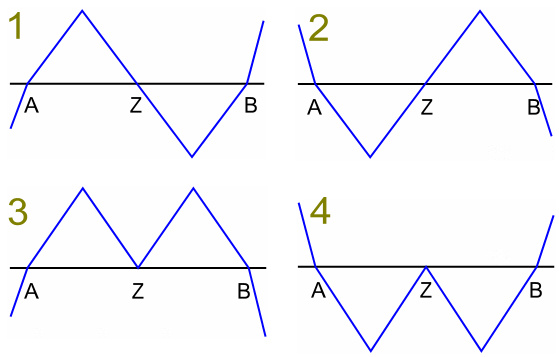
(Chart 2)

In diagram 1, two kill points A and B have an upward slope.  The zero point at Z is the exact mid-position with a downward slope.  If A and B describe note values, Z=(A+B)/2.

In diagram 2, two kill points A and B have a downward slope.  The zero point at Z is the exact mid-position with an upward slope.

In diagram 3, kill point A has an upward slope and kill point B has a downward slope.  The zero point at Z is the exact mid-position.  But Z doesn’t cut through the x-axis, it just dips down and touches it.

In diagram 4, kill point A has a downward slope and kill point B has an upward slope.  The zero point at Z is the exact mid-position.  It rises up to the x-axis and touches it without cutting through it.

There are 92120 kill points (including note 0), so there will be 92119 zero points.  That means the line crosses or contacts the x-axis 184239 times from note 0 to 6 inclusive.

Spike points

There is another set of kill points that I call ‘spike points’.  A spike point causes the energy line to dip down or up to zero, then revert to the previous value in a rectangular spike-like shape.  This diagram shows the concept:

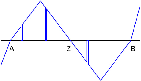
(Chart 3)

In this diagram, A and B are kill points and Z is a zero point.  There are three spike points shown: two dipping down to zero and a third dipping up to zero.  Spike points are extremely thin – typically around a billionth of a semitone.  For this reason they can be ignored in practise because it’s unlikely that a randomly chosen note will be one of them.  But it is worth investigating them because they reveal interesting information.

Spike points are calculated in a number of ways.  The first is via this formula:

sp = Mod6[slope*Log2[krat]^(2^pow)]      --(3)

Where:
sp  is the spike point
Mod6  is a modulus function that gives the remainder after dividing by 6
slope  will be either -1 or +1.
Log2  is a logarithm in base 2
krat  is a kill ratio from Table 2
pow  is an integer going from 0 to 3; i.e. one of: 0,1,2,3.

Example 1: krat=17, slope=1, pow=0:
sp = Mod6[1*Log[17]/Log[2]^(2^0)]
= Mod6[(1.230448921/0.3010299957)^1]
= Mod6[4.087462841]
= 4.087462841

Example 2: krat=9, slope=-1, pow=2:
sp = Mod6[-1*(Log[9]/Log[2])^(2^2)]
= Mod6[-(0.954242509/0.3010299957)^4]
= Mod6[-3.169925001^4]
= Mod6[-100.970835229]
= Mod6[-17*6+1.029164771]
= 1.029164771

In Example 1, the result of 4.087 is a number that we use in a 12-tone scale.  Except we didn’t do anything to convert it to a 12-tone scale, we just took the base 2 log of 17.  This is quite different from equation (1) where we convert to a 12-tone scale by multiplying a number in the range of 0 to 0.5 by 12 to get a number from 0 to 6.  Equation (3) doesn’t do this, it only takes modulus 6, where 6 is also a number in a 12-tone scale.  What this tells us is the 12-tone scale is fundamentally encoded in our brains.  This likely explains why it is preferred over other scale subdivisions.

In equation (3), slope doesn’t refer to a slope of any kind.  It is just a position marker that mirrors a result around the note 3.  Each positive has a negative that can be calculated by subtracting that number from 6 and visa-versa.  E.g. 4.087462841 has a negative of 6-4.087462841=1.912537159, and 1.029164771 has a positive of 6-1.029164771=4.970835229.

Spike points can also be generated using the secondary kill sources from Table 3.  Simply place those number in equation (3) in place of Log2[krat].

Example 3: slope=1, pow=3, Log2[krat]=1.41204798918928498
sp = Mod6[1*1.41204798918928498^(2^3)]
= Mod6[15.805041973]
= 3.805041973

There are also a set of secondary spike points.  They are generated from the first eight kill ratios, i.e. {3,5,7,9,11,15,17,23}.  The equation for generating them is this:

sp = 12*ModH[(ModH[slope*Log2[krat]^(2^xpow)] +1+6*xpow)^(2^pow)]  --(4)

Where:
sp  is the spike point
ModH  is a modulus function that gives the remainder after dividing by 1/2
Log2  is a logarithm in base 2
slope  will be either -1 or +1.
krat  is a kill ratio from the first 8 entries in Table 2
xpow  is an integer going from 1 to 3; i.e. one of: 1,2,3.
pow  is an integer going from 1 to 3; i.e. one of: 1,2,3.

Example:  krat=7, slope=1, xpow=2, pow=1
sp = 12*ModH[(ModH[1*Log2[7]^(2^2)]+1+6*2)^(2^1)]
= 12*ModH[(ModH[2.8073549221^4]+13)^2]
= 12*ModH[(ModH[62.11397007812]+13)^2]
= 12*ModH[13.11397007812^2]
= 12*ModH[171.976211210]
= 12*0.476211210
= 5.714534517

From this we would expect a total of 8*4*3*2=192 audible kill points to be generated.  But not all of them are: 27 don’t sound like kill points.  Looking over those that were excluded, it appears that the problem is a lack of precision.  When the Modulus function is used, it removes some of the leading digits and this requires more trailing digits to get the same accuracy in the final result.

Let’s look at the highest and most excluded/invalid result, which is from krat=23, slope=1, xpow=3, pow=3.  We’ll do the calculation using 21 digits of precision.  The first few steps are:
sp = 12*ModH[(ModH[1*Log2[23]^(2^3)]+1+6*3)^(2^3)]
= 12*ModH[(ModH[4.52356195605701287229^8]+19)^8]
= 12*ModH[(ModH[175325.200152252577670]+19)^8]

To take the modulus 1/2 of the inner portion requires subtracting 175325, which reduces 5 digits of precision:
sp = 12*ModH[19.200152252577670^8]
= 12*ModH[18468744811.01345795]

Taking modulus 1/2 of this requires subtracting 18468744811, removing a further 11 digits of precision:
sp = 12*0.01345795
= 0.1614954

The actual result correct to 9 decimal places is 0.161589448.  So only the first 4 digits of what we calculated are correct.  The modulus function has removed a lot of accuracy.

Now look at a result that’s also excluded, but by the least amount, which is from krat=7, slope=-1, xpow=2, pow=3.  Again doing the calculation with 21 digits of precision we get:
sp = 12*ModH[(ModH[-1*Log2[7]^(2^2)]+1+6*2)^(2^3)]
= 12*ModH[(ModH[-2.80735492205760410744^4]+13)^8]
= 12*ModH[(ModH[-62.1139700781162342997]+13)^8]
= 12*ModH[13.3860299218837657003^8]
= 12*ModH[1030894758.74804851463]
= 12*0.24804851463
= 2.976582176

The actual result to 9 places should be 2.976582174.  We have lost a lot of precision due to the modulus function and only the last digit is off by 2.  But neither calculated result sounds like a kill point.

Next we’ll look at a result that IS included, but only just, which is krat=7, slope=1, xpow=2, pow=3 – same as the previous but with negative ‘slope’.  Again with 21 digits of precision we get:
sp = 12*ModH[(ModH[1*Log2[7]^(2^2)]+1+6*2)^(2^3)]
= 12*ModH[(ModH[2.80735492205760410744^4]+13)^8]
= 12*ModH[(ModH[62.1139700781162342997]+13)^8]
= 12*ModH[13.1139700781162342997^8]
= 12*ModH[874728964.352283548305]
= 12*0.352283548305
= 4.227402580

This matches the actual result to 9 places and sounds just like a kill point.

What this suggests is our brain is doing calculations using something slightly higher than 21 digits of precision.  But it’s highly unlikely our brain works in base 10.  It’s far more likely to work in base 2 (binary) like other computers.  2 to the power of 70 is 10 to the power of 21.07, i.e. just over 21 digits.  Therefore it’s possible our brain uses a 70 bit processor of sorts.

There’s also another group of spike points calculated according to this formula:

sp = 12*ModH[(ModH[slope*(prev/12+7)^(2^xpow)] +1+6*xpow)^(2^pow)]   --(5)

Where:
prev  is a spike point previously calculated from equation (4) or this equation (5)
slope  will be either -1 or +1.
xpow  is an integer going from 1 to 3; i.e. one of: 1,2,3.
pow  is an integer going from 1 to 3; i.e. one of: 1,2,3.

This equation operates on the results of equation (4), but also on results previously generated by the same equation.

Example.  Take the earlier result of 5.714534517 generated by krat=7, xpow=2, pow=1.  Now feed that into equation (5) using slope=1, xpow=1, pow=1.  For this we will instead use the value calculated using 21 decimal precision, which is 5.7145345167349476:
sp = 12*ModH[(ModH[1*(5.7145345167349476/12+7)^(2^1)]+1+6*1)^(2^1)]
= 12*ModH[(ModH[55.893734052461294]+7)^2]
= 12*ModH[54.6673032385257]
= 12*0.1673032385257
= 2.0076388623084

We now take this and feed it through equation (5) again with the same parameters to get:
sp = 12*ModH[(ModH[1*(2.0076388623084/12+7)^(2^1)]+1+6*1)^(2^1)]
= 12*ModH[(ModH[51.370235712981]+7)^2]
= 12*ModH[54.3203744649]
= 12*0.3203744649
= 3.8444935788

As can be seen, precision is steadily dropping with each iteration.  But we still have 10 decimals of accuracy and the results still confirm as spike points.  The next iteration of this will fail.

Equation (5) can be applied over and over until the accuracy drops below 9 decimals, at which point the process stops.  As it happens, no result from equation (4) can be extended more than three times using equation (5) because accuracy won’t allow it.  Using equations (4) and (5) allows 1135 spike points to be created.

Once the spike points are generated, they can be replicated via equation (2).  But there is a small difference in that pow can go from 1 to 6; i.e. 2^pow will be one of: 2,4,8,16,32,64.

Example:  Take the first spike point example and use krep=-13 and pow=6.  Equation (2) gives:
krep = 4.087462841*2^(-13/64) = 3.550643747
Which sounds as a spike point.

There is one more spike point source, which is 9*2^(-7/4)= 2.675716009.  This can be fed into equation (3) in place of Log2[krat].  It can also be replicated via equation (2).  One such replication using krep=3 and pow=2, gives the simple result 4.5.  This is the example mentioned in the introduction.

As a result of following these rules we generate:
. 124043 primary spike points
. 146422 secondary spike points
. 943 spikes from the 9*2^(-7/4) source
Altogether a total of 271408 spike points.

That’s a huge number – almost three times the number of regular kill points.  But as mentioned, these are so thin they can be ignored in practise.

There may be additional spike points that aren’t included here.  Finding spike points is often a matter of stumbling upon one of them, and then tracing it back to its source.

Further information about spike points, along with very interesting behaviour that occurs around them, can be found in a separate article:

Spike Points in Detail

Inversion notes

In certain situations the comparison between two notes can be reversed by the inclusion of an ‘inversion note’.

An inversion note is a note that sits within the upper-half region between two kill points.  It runs from the zero point to the next kill point above.  These charts describe it:

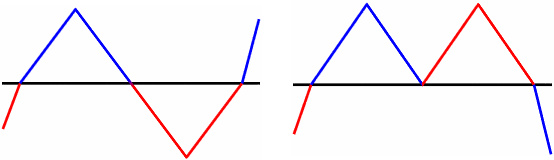
(Chart 4)

In both charts the inversion region is the red section that goes from the zero point to the next kill point.  It doesn’t matter what the leading slope is or whether the zero point crosses the x-axis.

But there is a twist to this rule: if the lower kill point is greater than 3.012147 and the kill points either side have opposite slope, the inversion region is instead the lower portion (below the zero point).  These charts describe it:

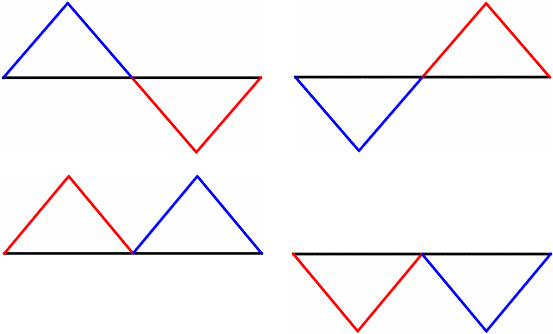
(Chart 5)

In all four charts the regions shown are above 3.012147.  When the kill-point slopes are both upward or both downward, the inversion region (red section) is the second half.  But when slopes are opposite, the inversion region is the first half.

The number 3.012147 is calculated from one of the secondary kill sources and is more accurately 12*ModH[1.41204798918928498^8]*2^(-9/32)=3.012146993.

Inversions are important as follows:  If the upper note in the lower-half octave is an inversion, and the average of the middle notes is an inversion, the relationship between note 0 and the upper note becomes opposite.

Note 5 is an inversion and so is note 3.  If you were to play 0 and 5, 5 would be base.  But if you were to play 0,3,5, note 0 would instead become base because 3 inverts 5.  And if you were to play 0,2,5 or 0,4,5, note 5 would still be base because notes 2 and 4 are not inversions.  But if you play the four notes: 0,2,4,5, note 0 would be base because the average of 2 and 4 is 3, which is an inversion.

The reason note 5 is an inversion note is not because it is the natural base of 0 and 5, but because it is greater than 3.012147 and sits within the lower-half region of two surrounding kill points that have opposite slope.  Another inversion note is 5.00232.  The base of 0 and 5.00232 is 0, but when played with note 3, 5.00232 becomes base instead of 0.

On the 12-tone equal-temperament scale, only two notes are inversions: 3 and 5.  But we need to consider other possibilities because certain groups of middle notes also have an average that is an inversion.  There are three others:

1.5, caused by average of notes 1 and 2
3.5, caused by average of notes 3 and 4
8/3 (~=2.66667), caused by average of notes 1,3,4

So if working on a 12-tone scale, the values {1.5, 8/3, 3, 3.5, 5} can be saved in a table rather than consulting a large kill-point table.

Note energy flipping

Up till now, energy charts for notes are being depicted as zigzags that rise and fall in straight lines between kill or zero points and nearby peaks.  While this triangular shape is basically correct, it is only true as far as magnitude.  In reality, the energy flips rapidly back and forth between positive and negative regions.  This is too complicated to get into here and is discussed in a separate article:

Note Energy Flipping

App for calculating kill points and energies

Here is an interactive application that calculates kill points:

Calculate Note Energy    (opens in new tab)

This is quite extensive.  It generates kill points and spike points.  It then allows entry of a note value and shows its location within a table of surrounding kill and spike points, as well as the nearby peaks and zero point.  The table can be scrolled up and down.

It also gives the note energy and inversion status.  The note energy is adjusted for flip intervals.  Finally, it shows the activation ranges for kill and spike points.

The calculations are done in JavaScript.  The source for this can be studied and followed in debug mode to understand exactly how the calculations are done.

Inner-note comparisons

Now that the method for comparing two notes has been described, we can move to three and above.

The comparison process is done in half octaves.  Notes in the range 0 to less than or equal to 6 are treated differently from the notes greater than 6 and less than 12.  Let’s first consider the case of all notes being in the lower octave.

There are two types of comparisons.  The first is the ‘outer note comparison’, which is the comparison between the lowest note (usually note 0) and the highest note in the lower half-octave.

The second is the ‘inner note comparison’.  This is the comparison between the lowest note and another note in the lower half-octave but below the highest.

For example, suppose we have notes 0,2,3,4,5.  The outer comparison will be the 0-5 pair.  There are three inner comparison pairs: 0-2, 0-3, and 0-4.  So there can be multiple inner comparisons but only one outer comparison.

We have already described how to do outer comparisons and have seen they are rather complicated.  Fortunately the inner comparisons are much simpler.  They work as follows:

If the inner note is above the average of the outer notes, it is lower energy than note 0, otherwise note 0 is base.  Stated more formally, suppose we have notes 0,a,b where a and b are <6:

If a<b/2 , note 0 is lower than a
If a>b/2 , note 0 is higher than a
If a=b/2 , note 0 and a are equal
(Rule List 1)

In the case of our 0,2,3,4,5 example, the average of 0 and 5 is 2.5.  Therefore note 0 is the base of the 0-2 pair, whereas notes 3 and 4 are the base of the 0-3 and 0-4 pairs respectively.  If there was an inner note of 2.5, both it and note 0 would be equally base.

The 0-6 interval

The 0-6 interval – representing C to F# – is a special case.  As mentioned, note 6 is a kill point, which means any notes played within the interval 0-6 will seem dead… in fact this is not fully true.  As will be later shown, kill points don’t activate until entering the secondary buffer.  Until then there will be a brief interval in which the interior notes can be compared as follows:

If the inner note is below 3, it is lower energy than note 0, otherwise note 0 is base.  Stated more formally, suppose we have notes 0,a,6, where a<6:

If a<3 , note 0 is higher than a
If a>3 , note 0 is lower than a
If a=3 , note 0 and a are equal
(Rule List 2)

Basically, it follows the same rules of the inner-note-comparisons, but with directions reversed.

Example: take the notes 0,2,3,4,5,6.  Note 0 will be higher than 2, equal to 3, and lower than 4 and 5.

Influence from the upper half-octave

Thus far we’ve only considered situations where all notes are in the lower half-octave.  Now let’s look at the upper half, which includes notes above 6 and less than 12.

While no direct comparisons are made between notes in the lower and upper, what the upper half can do is modify the comparisons made in the lower half.  Namely, it can reverse or neutralise them.

The simplest situation is when is there is only one note in the lower-half, i.e. note 0, and one or more notes in the upper.  This situation reveals no comparison rules.

The next situation is when there are two or more notes in the lower-half.  Here is where it becomes complicated.  There are two important points to consider:

 .  The only thing that matters is the average value of the outer notes in the upper half-octave.  E.g. if we have notes 7, 9, 10, this average will be (7+10)/2=8.5, and note 9 won’t affect it.
 .  In the upper-half there is a special region running from 12-3/sqrt(2) (i.e. 9.878679656440358) to 11.27183739887399.  If the upper-half average is within this region, all comparisons in the lower half-octave will be nullified.  Let’s refer to this as the Blocking Zone.  In the 12-tone scale, this includes notes 10 and 11.

Now to look at the specifics.  There are four situations to consider:

 .  Outer note without inversion
 .  Outer note with inversion
 .  Inner note or 0-6 interval
 .  Inner middle note without inversion

1.  Outer note without inversion

This refers to the comparison between note 0 and the highest note in the lower half-octave, and when no inversion process is taking place within it.  If the upper average is an inversion, the comparison will be reversed.

More formally, suppose we have five notes: 0,a,b,c,d,e where a and b are in the lower half-octave and c,d,e are in the upper-half.  Let B1=(c+e)/2 – (observe that B1 excludes d).

If B1 is within the Blocking Zone,
  Note 0 and b are equal
Else If B1=inversion,
  The comparison between 0 and b is reversed
Else
  The comparison between 0 and b remains the same
(Rule List 3)

Example:  Take notes 0,3,4,8,10.  Without the upper octave, 0 would be base of the 0-4 pair.  Within the upper octave, the average is (8+10)/2=9.  9 is an inversion because 12-9=3 and 3 is an inversion.  Therefore the comparison reverses and 4 is instead the base of 0-4.

2.  Outer note with inversion

The next situation involves an outer note that has been inverted.  This inversion can be undone (i.e. re-inverted) as follows:

If the average of the notes in the upper half-octave is less than 9, we can undo the inversion rule.  This number 9 isn’t fixed, it decreases by one semitone for every additional middle note in the lower half-octave.  For two middle notes it is 8, for three it is 7.  For four or more notes, the cancellation rule disappears.

To state more formally, suppose we have a group of notes: 0,b1,b2,…,bn,c,d1,d2,..dm.  These are in ascending order with c<6 and d1>6.  Let B1 be the average B1=(b1+b1+…+bn)/n, B2=10-n, and D1 the average D1=(d1+dm)/2.  If c is an inversion and B1 is an inversion:

If D1 is within the Blocking Zone,
  Note 0 and c are equal
Else If n<4,
  If D1>B2 the base of 0 and c is the base of 0 and c when played alone
  If D1<B2 the base of 0 and c is the opposite of the base of 0 and c when played alone
  If D1=B2 the base of 0 and c is neither, i.e. 0=c
Else
  The base of 0 and c is the opposite of the base of 0 and c when played alone
(Rule List 4)

Example:  Consider notes 0,3,5,9.  Starting with just 0 and 5, 5 is base.  Now 5 is an inversion, so adding note 3, which is also an inversion, makes note 0 the base of 0-5.  We then add note 9, which is also an inversion because 12-9=3, and now note 5 is again base.  So effectively we have a double inversion process, which cancels the first inversion.

An interesting observation is that this re-inversion rule refers to intervals in the 12-tone scale.  Just as with the spike points, this is further evidence that the 12-tone scale is built into our brains.

3.  Inner note or 0-6 interval

The next situation covers both inner notes both within 0-X interval, where X<6, and the 0-6 interval.  Comparisons can be reversed as follows:

If the upper outer-notes average is equal to an inversion note, the comparison between note 0 and the inner note will be reversed, but only if that inner note is above the average of the highest lower note.

More formally, suppose we have five notes: 0,a,b,c,d,e where a is in the lower half-octave, b is less than or equal to 6, and c, d, and e are in the upper-half.  Let B1=(c+e)/2.

If B1 is within the Blocking Zone,
  Note 0 and a are equal
Else If B1=inversion and a>b/2,
  The comparison between 0 and a is reversed
Else
  The comparison between 0 and a remains the same
(Rule List 5)

Examples:  Suppose we have the notes 0,4,5,X, where X is in the upper half-octave.  If X wasn’t there, according to Rule List 2, note 4 would be lower than 0.  For all other values:

If X=7, this corresponds to inversion note 12-7=5.  Therefore 4 is higher than 0.
If X=8, this isn’t an inversion and is less than 9.88.  Therefore 4 is lower than 0.
If X=9, this corresponds to inversion note 12-9=3.  Therefore 4 is higher than 0.
If X=10, this is higher than 9.88.  Therefore 4 is higher than 0.
If X=11, this is higher than 9.88.  Therefore 4 is higher than 0.

4.  Inner middle note without inversion

The final situation covers an inner note at the mid-point, and a non-inversion upper average.

If the inner note is at the exact mid-point of the lower half octave and the upper outer-notes average is not equal to an inversion note, the lowest note will be base of the mid-point note.

More formally, suppose we have five notes: 0,a,b,c,d,e where a is in the lower half-octave, b is less than or equal to 6, and c, d, and e are in the upper-half.  Let B1=(c+e)/2.

If B1 is outside the Blocking Zone  AND  B1<>inversion,
  Note 0 is the base of 0 and a
Else
  Note 0 and a are equal
(Rule List 6)

Examples:  Suppose we have the notes 0,2,4,X, where X is in the upper half-octave.  If X wasn’t there, notes 0 and 2 would be equal.  For other values:

If X=8, this is not an inversion note.  Therefore note 0 will be base of 0 and 2.
If X=9, this is an inversion note.  Therefore notes 0 and 2 will be equal.

Secondary memory buffer comparisons

As mentioned, our brains appear to have two high-accuracy memory buffers – one covering the most recent 7 seconds, which we’ll call the ‘primary buffer’, and another covering the 7 seconds before it, which we’ll call the ‘secondary buffer’.  This second buffer has three effects, as follows:

1.  Applying kill points

The first effect is to apply the cancelling action of kill points.  When a note corresponding to a kill point is contained in the secondary buffer it nullifies all notes in the lower half-octave of the primary.  When the kill point is in the primary buffer but not the secondary, it will sound equal to note 0 but it won’t affect other notes.

Example: select the notes 0,1,4, and the kill point 4.967415943.  Start by briefly playing 4.967415943 then alternating between 0,4 and 0,1.  For the first 7 seconds we hear 0 as base of both 1 and 4.  Then around the 7 second mark, all notes become equal.

What happened is that the kill point was initially in the primary buffer and had no effect on the 0,1 and 0,4 comparisons.  Then the kill point moved from the primary to the secondary buffer where it nullified the comparisons.  After 14 seconds, the kill point will move out of the secondary buffer and the comparisons can be heard again.

Spike points act a bit differently.  They nullify other notes for three buffer lengths.  So, for example, if we played the spike note 4.5, it would nullify all the comparisons for around 21.5 seconds.

There are two further considerations regarding kill points:
  1.  A kill point from the lower half-octave of the secondary buffer won’t be applied
      if there are notes in the upper half-octave of the primary buffer.
  2.  A kill point from the upper half-octave of the secondary buffer won’t be applied
      if there are three or more notes in the lower half-octave of the primary buffer.
These considerations apply only to kill points, not spike points.

2.  Nullifying the outer note

The second thing the secondary buffer can do is to nullify the comparison in the primary buffer between note 0 and the highest note in the lower half-octave, also known as the ‘outer note’.  This happens when there are one or more notes anywhere in the secondary buffer, and no notes in the upper half-octave of the primary buffer.

Example: select the notes 0,4,9.  Start by alternating between 0 and 4 and hear note 0 is base.  Then play note 9.  Then continue alternating between 0 and 4, but now hear 4 is base.  After 7 seconds, 0 and 4 sound equal.  Then after 14 seconds, 0 goes back to being base.

What happened is that note 9 reversed the 0-4 comparison, because 9 is an inversion note.  Then note 9 moved to the secondary buffer and nullified the 0-4 pair.  Then note 9 moved out of the secondary buffer and lost all effect.

But there are two situations where cancelation doesn’t occur.  The first is when the lower average of the secondary buffer is equal to half the outer note in the primary.  The second is when the upper average of the secondary buffer is equal to 12 minus the outer note.

More formally, suppose the primary buffer has notes 0,a,b, where a and b are <6.  And the secondary buffer has notes d,e,f,g,h,i, where d,e,f are <=6 and g,h,i are >6.  Let B1=(d+e+f)/3 and U2=(g+i)/2.

If (B1=b/2  OR  U2=12-b)  AND  U2 is outside the Blocking Zone,
  The comparisons between 0 and a, and 0 and b, are normal
Else
  The comparison between 0 and a is normal
  The comparison between 0 and b is nullified, i.e. 0=b
(Rule List 7)

This rule only affects the outer note comparison and only comes into effect when there are no notes in the upper half-octave of the primary buffer.  If there are no notes in the lower half-octave of the secondary buffer, ignore the reference to B1, and if there are no notes in the upper half-octave of the secondary buffer, ignore the reference to U2.

Example:  Suppose the primary buffer contains 0,1,4.  With an empty secondary buffer, note 0 would be base of both 1 and 4.  Now put into the secondary buffer: 1,3,7,9.  The average of this lower half-octave is (1+3)/2=2. This matches the half of the outer note 4/2=2.  Therefore it won’t nullify the 0-4 relationship.  Next, the average of the secondary upper half-octave is (7+9)/2=8. This matches the inverse of the outer note 12-4=8.  Therefore it also won’t nullify the 0-4 relationship.  But if any single note of this secondary buffer was moved, note 0 and 4 would become equal.

3.  Reversal of comparisons

The third thing the secondary buffer can do is to reverse the comparisons made in the primary buffer as follows:

If the magnitude of the energy of the average of the outer notes in the upper half-octave of the secondary buffer is higher than the magnitude of the energy of the average of the outer notes in the upper half-octave of the primary buffer, all comparisons in the lower half-octave will be reversed.

Example:  Take the notes 0 and 5, for which 5 is base.  Now take two notes in the upper octave: 9.000581 and 9.000591.  It can be observed that 9.000581 has lower energy than 9.000591, when comparing them with note 0.

We start by alternating between notes 0 and 5, and confirm 5 is base.  We then play note 9.000591.  We then pause for 7 seconds, then play note 9.000581.  We then alternate between notes 0 and 5 and hear that note 0 is base instead.  We continue alternating and find that after another 7 seconds, neither is base.  We continue for another 7 seconds and find 5 is base.

Why did the base move back and forth?  When 9.000591 was in the secondary buffer it caused the 0-5 relationship to reverse, making 0 base.  After 7 seconds, 9.000591 exited the secondary buffer and no longer had influence.  But now the three other notes 0, 5, and 9.000581 entered the secondary and the primary had 0 and 5.  This made 0 and 5 equal according to Rule List 7.  After another 7 seconds, 9.000581 left secondary buffer, leaving only 0 and 5 in both buffers, which meant 5 was again base.

Notice it refers to the magnitude of the energy rather than just the energy.  This means we disregard the energy sign (positive or negative) and look at absolute value.  E.g. -0.8 is a lower energy than 0.4, but it’s of higher magnitude.

This reversal applies to all comparison types.  Some examples:

 .  For an ‘inner note’ comparison, if we select notes 0,4,5, note 4 will sound base relative to note 0.  But after putting it through a process like the above, note 0 will instead be base.
 .  For an inversion, if we select notes 0,3,5, note 0 will sound base relative to note 5.  But after putting it through the above process, note 5 will instead be base.
 .  For a 0-6 interval, if we select notes 0,4,6, note 0 will sound base relative to note 4.  But after putting it through the above process, note 4 will instead be base.

It is a bit more complicated because we also need to include the energy of the average of the notes in the lower half-octave of the secondary buffer and then average this with the upper average.

More formally, suppose we have ten notes: 0,a,b,c,d,e,f,g,h,i where a,b,c is in the lower half-octave of the primary buffer, d and e are in the upper-half of the primary, f and g are in the lower-half of the secondary, and h and i are in the upper-half of the secondary.  Let B1=(d+e)/2, C1=(f+g)/2, and C2=(h+i)/2.  Also let BE1=Abs[energy of B1], CE1=Abs[energy of C1], CE2=Abs[energy of C2], and CE3=(CE1+CE2)/2.

If BE1=CE3  OR  either of B1 or C2 is within the Blocking Zone,
  The comparisons between 0 and b, and 0 and c, are neutralised
Else If BE1<CE3,
  The comparisons between 0 and b, and 0 and c, are reversed
Else
  The comparisons between 0 and b, and 0 and c, are normal
(Rule List 8)

Rotating notes

Up until now we have been comparing the note at the bottom of the scale with one or more of the notes above it.  How do we compare the other notes?  This will be done using note rotation.

To rotate a group of two or more notes, do the following:

1. Look at the distance between the lowest note on the scale and the next highest note.
2. Take the lowest note on the scale and add 12 to it, i.e. move it up an octave.
3. Subtract the distance from step 1 from all notes.

For example, consider the notes C,E,G which are numerically 0,4,7.  The distance between the first and second is 4-0=4.  We add 12 to the lowest note: 0+12=12, and move it to the end of the list.  This gives 4,7,12.  Now subtract 4 from all of these, yielding 0,3,8.

Repeating this process gives 3,8,12, yielding 0,5,9.  Repeating it again returns to the original 0,4,7.  In other words, C,E,G rotates to C,D#,G#, which rotates to C,F,A, which rotates to the original C,E,G.  For a group of N notes there will be N possible rotations.

For each rotation we will determine the relationship of the note at the bottom to some of the other notes in the lower half-octave.  We will determine whether the bottom note is of higher, lower, or equal energy relative to those other notes.  Each rotation will reveal zero or more comparisons.

Now an important rule here is that the first rotation is strict and its comparison rules must be followed.  Comparison rules stemming from other rotations will only be included if they don’t contradict those in the first rotation.
(Rule List 9)

The general method

In summary, the method for comparing a group of notes is as follows:

Examples

With the rules now in place, we’ll do some examples.  These will assume the secondary buffer is empty, which requires all notes be played and listened to within 7 seconds.

Example 1

The first example uses the notes 0,4,7, which make up the chord C,E,G.  The rotations for this were mentioned earlier but here they are in numerical form:
0,4,7
0,3,8
0,5,9

But we wish to preserve the original note so let’s rewrite the above so each number is followed by the original note letter:
0C,4E,7G
0E,3G,8C
0G,5C,9E

In the first rotation suggests C<E, but note 7 in an inversion so according to Rule List 3, this reverses to E<C.

The second rotation tells us E<G because note 0 is the base of 0-3 and note 8 isn’t an inversion.

The third rotation tells us G<C because note 9 is an inversion.

So we have E<C, E<G, and G<C.  The only arrangement that satisfies this is E,G,C.  This means E is base, G is second best choice and C is furthest from base.

This can be confirmed by listening but needs to be played and tested within 7 seconds.  If longer than that, the upper half-octave notes may end up in both the primary and secondary buffers.  This will cause all comparisons to be neutralised (see Rule List 9), leaving the result C=E=G, i.e. all are equally base.


Example 2

The second example will be notes C,E,F, which are described as 0,4,5.  The three rotations are:
0C,4E,5F
0E,1F,8C
0F,7C,11E

In the first  rotation, all notes are in the lower half-octave so we refer to Rule List 5.  4>5/2 so the second rule tells us 0C>4E, which we record as E<C.

The first rotation also allows comparison of 0C and 5F, using the two-note comparison, which says 5F<0C.  5F is an inversion so this comparison has the potential to be reversed, except that the middle note 4E isn’t an inversion so the comparison remains.  We record this as F<C.

In the second rotation, there are two notes in the lower half-octave and one in the upper.  The upper note 8 is not an inversion and Rule List 3 tells us 1F<0E, or F<E.

The third rotation has only one note in the lower half-octave and yields no comparison rules.

So we have E<C, F<C, and F<E.  This is one arrangement that satisfies these rules: F,E,C.  So F is base, E is second best, and C is worst.  This is confirmed by listening.


Example 3

The third example will be notes C,D,E,F, which are described as 0,2,4,5.  The four rotations are:
0C,2D,4E,5F
0D,2E,3F,10C
0E,1F,8C,10D
0F,7C,9D,11E

The first rotation reveals the lower half-octave’s outer notes 5F<0C (via two-note comparison).  But the average of the middle notes 2D and 4E is 3D#, which is an inversion, so we instead take the reverse: 0C<5F.  The first rotation also reveals inner note comparisons 0C<2D and 4E<0C.

In the second rotation the upper average is 10, which is above the special location ~9.88 and nullifies all comparisons in the lower, giving 0D=2E and 0D=3F.

In the third rotation the upper average is 9, which is and inversion, making the lower comparison 0E<1F.

The forth rotation reveals no information.

So we have:  C<F, C<D, E<C, D=E, D=F, E<F.  Putting aside the D=E, the only sequences of notes that satisfies this are E,C,D,F and E,C,F,D.  But what about the D=E rule?  It can’t be followed because C is in-between D and E.

Now refer to Rule List 9 which instructs us to reject comparisons from higher rotations that conflict with those in the first rotation.  The D=E rule came from the second rotation so we reject that, but we’ll keep the other D=F rule because it doesn’t conflict.

So we are left with E,C,D=F.  This means E is the best choice for base, C is second, and D and F are equally third.  This is confirmed by listening.  If we were to rearrange the notes via rotation, a different note might be base.


Example 4

Consider the set of notes: C,D,E,F,G,A.  Without going through details, the comparisons from each rotations are:

1st: F=C, C<D, E<C
2nd: D<G, D<E, D<F
3rd: E<A, E<F, E<G
4th: A<F, G=F
5th: G<C, G<A
6th: D<A, A<C

(How does F=C?  C,F is an inversion and the average of the inner D,E pair is 3, which is also an inversion, so refer to Rule List 4.  The average of the upper half-octave is D1=8, and the number of inner lower half-octave notes is 2, making B2=10-2=8.  So D1=B2 and line 6 of that rule list tells us C and F are equal.)

There’s no arrangement of notes that satisfies all these rules.  So we refer to Rule List 9 and look only at the first rotation: F=C, C<D and E<C.  There’s two arrangements of these notes that satisfy this: E,C,F,D and E,F,C,D.  This means E is the best choice for base, C and F are equal second best, and D is least.


Example 5

Consider the notes C,D,F,G,A,B.  The rotations reveal comparisons:

1st: C<F, C<D
2nd: G<D, D<F
3rd: B=F, G<F, F<A
4th: G<C, G<A, G<B
5th: A<D, A<B, A<C
6th: F=B, C<B, D=B

There’s no arrangement that satisfies all these rules.  So we look at the first rotation: C<F, C<D.  There’s one arrangement for this: C,D,F.

Now we’ll look at other rotations for non-conflicting comparisons that can assist with those in the first rotation.  One of these is D<F, which doesn’t contribute anything.  But there’s three others: G<D, G<F, and G<C.  They tells us that G is lower energy than all of C,D,F and needs to be at the front of the list.  So our result is G,C,D,F, making G base, C second best, D third, and F least best.  An interesting result!  A good way to confirm this is to play all the notes twice, then finish in reverse least-to-best base choice: F,D,C,G.  By doing this you can hear the energy slowly descending, which gives the pleasing effect of music ‘winding down’.


Example 6

Now to do the full C-major scale: C,D,E,F,G,A,B.  The comparisons from each rotations are:

1st: C<F, C<D, C<E
2nd: D<G, D<E, D<F
3rd: E<A, E<F, E<G
4th: B=F, G<F, A<F
5th: G<C, G<A, G<B
6th: A<D, A<B, A<C
7th: F=B, C<B, D=B, E<B

The first rotation tells us C<F, D<C, C<E.  We can also find non-conflicting rules from other rotations: D<F, E<F, E<G, A<F, G<A, F=B.  The arrangement that fits these is C,D,E,G,A,F=B, making C base, D the second choice, and E,G,etc. trailing that.  This order is confirmed by listening and shows this scale deserves the name “C-major”!


Example 7

For the final example, consider the notes C,D,F,G,A,C+, where C+ is the note one octave higher than the first C.  We’ll start of by ignoring the final C+ for the moment.  The rotations reveal comparisons:

1st: F<C, C<D
2nd: G<D, D<F
3rd: F<A, F<G
4th: G<C, G<A
5th: D=A, A<C

The first rotation reveals F is base, followed by C then D.  Other rotations tell us F<G and G<C, which tells us G is between F and C.  Therefore the base is F.  If we listen to the notes played in the order C,D,F,G,A, and without the final C+, we can confirm F as base.

But if we instead play the full sequence C,D,F,G,A,C+, now G is base, and F isn’t.  What happened?

What happened is the lower C got replaced by the higher C+.  So we are now hearing the sequence D,F,G,A,C+.  In this scale, D is at the bottom, and the first rotation becomes the old 2nd rotation, namely G<D, D<F.  What this tells us is G is base, followed by D then F.

But, if we play the full sequence and return to the lower C, namely C,D,F,G,A,C+,C,  F once again becomes base.  This reveals an important rule:

When notes separated by an integer number of octaves are played, the most recent of them is the one considered for scale analysis.
(Rule List 10)

App for calculating base notes

Here is an interactive application that calculates base notes:

Calculate Base Notes in a Scale    (opens in new tab)

A list of notes can be entered.  When clicking ‘Get base notes’, it does the calculations, then displays a list of base notes in best-to-worst order.  The notes can be played back in the order entered, followed by the base notes in worst-to-best order.  This gives a ‘winding down’ effect to the ideal base.

Notes in both the primary and secondary buffers can be entered.  Non-integer note values can be used.  This requires a kill point table be generated.  The 12-tone scale note energies are stored and don’t require the large kill point table.  The app also allows for calculation of acoustic instrument scales (see later section).

Long-term memory buffers

As mentioned earlier, in addition to the five 7-second memory buffers there are also some longer-term buffers that remember frequency information with high accuracy.  The first runs from 169681 milliseconds to 339362 milliseconds – approximately 2:50 to 5:39 minutes.   The second runs from 339362 milliseconds to 509043 milliseconds – approximately 5:39 to 8:29 minutes.

The first of these compares notes within the lower half-octave, and the second compares notes between the lower and upper half-octave.

The first buffer works as follows.  Suppose we have notes 0 and A, where A is in the lower half-octave and they are unequal – i.e. alternating between 0 and A shows one of them to be base.  If the non-base note is located in the first buffer, the comparison between 0 and A disappears and they will sound flat.

Example:  Take notes 0 and 3.000037, for which note 0 is a strong base.  Briefly play the non-base note 3.000037.  Then wait two and a half minutes, i.e. listen to 2:30 of silence.  Now start alternating between the two notes and observe that note 0 is base.  When the 2:50 mark is reached, suddenly the notes will sound flat, with neither being base.  Continue alternating.  When the 5:39 mark is reached, now note 0 will sound as base again.

The second buffer works the same way but for notes in the upper half-octave.

Example: Take the notes 0 and 8.999963, for which 8.999963 is a strong base.  Briefly play non-base note 0, then listen to 2:30 of silence.  Now start alternating between those notes and observe 8.999963 is base.  Continue doing that past 2:50 and observe that 8.999963 is still base.  Continue doing that past 5:39 and observe that the notes now sound flat, with neither being base.  Continue doing that beyond 8:29 and observe that 8.999963 is base again.

Acoustic vs Digital instruments

Thus far, all the comparison rules have assumed our instrument is perfectly tuned.  This will be true for digital instruments but not for acoustic ones like stringed pianos.

As mentioned, the requirements for tuning are very precise.  Even a small change of a thousandth or millionth of a semitone can yield different results.  It will be impossible to tune an acoustic piano with that level of accuracy.  Thus, every acoustic piano will not match the results of Table 1, and every octave on a given piano will be different from each other.  In which case, how can we hope to determine scale bases at all?

It appears that acoustic instruments don’t obey two-note comparison rules.  If you alternate between two notes, neither seems to be favoured as base, or the apparent base switches back and forth.  This is likely because the generated frequency is imperfect and moves around.

But the rules for three notes or more are followed.  That is, if a middle note is above the mid-point of two outer notes in the lower half-octave, it will be base, otherwise the lower note will be base.  For example, if we have notes C, E and F, we can say for certain that E will be base of C and E.

For outer notes in the lower half-octave, these will be considered indeterminate rather than equal.  This means we won’t generate any comparison rules for them, which means that the relationship between them can be determined from other rotations.  We also don’t need to take into consideration things like inversions, kill points and spike points, as these don’t appear to come into effect.  One thing that will come into effect is the Blocking Zone, since this is a broad region covering notes 10 and 11, and will force the relationships within the lower half-octave to be equal.

An important point of consideration is the 0-6 interval.  On a digital instrument, note 6 counts as part of the lower half-octave.  But on an acoustic instrument, it will be either slightly higher or lower than that.  If lower, it will be part of the lower half-octave, and if higher, it belongs in the upper-half.  A small change in location will completely alter the calculations.  One way to deal with this is to avoid the 0-6 interval, which is what the major and minor scales do.

Another point of consideration is when an inner note is at the mid-point of outer notes.  For example, take the notes C, D and E.   On a digital instrument D, is at the exact middle and will be considered equal to C.  But on an acoustic instrument, D will either be slightly higher or lower than the mid-point.  So at some keyboard locations, D will sound as base, and other locations, C will be base.  In this situation we need to consider the relationship between the mid-note and bottom-note as indeterminate.

As a result of this analysis, we will likely end up notes that have no relationship to other notes on the scale.  So what we will do is sort those notes to make the lower frequencies as base.

Further observations

This concludes the main purpose of this paper, i.e. how to determine the base note.  But there are other points worth mentioning.


1.  Minimum duration

The minimum amount of time for a note to play in order to take effect appears to be 65 milliseconds.  E.g. take the note pair 0 and 3.000037.  For these notes, 0 is a strong base.  Now include the note 4.5, which is a kill point.  In order to neutralize the note pair 0 and 3.000037, note 4.5 needs to sound for at least 65 milliseconds.  If it sounds for less than that, e.g. 64 milliseconds, note 0 will be base.  This also holds true for other comparison types including inversion notes.

This 65ms refers to the sum of durations of the same note played over the past 7 seconds.  E.g. if we were to play a kill point three times, each for 25ms, that would be a total of 75ms, which means it would take effect, even if other notes were played in-between those repetitions.


2.  Effectiveness of the JND

Kill points are effective even when below the Just Noticeable Difference (JND).  Take the kill point 0.040004122 and the zero point 0.040018222.  Both are below the JND of 0.1 semitones and sound indistinguishable from note 0.  But the kill point will nullify larger note intervals such as 0,3.000037 whereas the zero point does not.

Inversion notes are also effective when below the JND.  E.g. take the non-inversion note 0.040011 and the inversion note 0.040025.  Both of these are below the JND of 0.1 and are indistinguishable from note 0 and each other.  When the non-inversion note is played with the notes 0 and 5, 5 is base.  But when the inversion note is played with 0 and 5, 0 is base.  This suggests the JND is something artificially imposed by our brains, rather than a limitation of our ears.


3.  Merging of nearby notes

A note may merge into a note that immediately follows if the distance them is less than about 1.116 semitones.

Suppose we have four ascending notes: 0,A,B,C.  A and B are kill points relative to 0 but C isn’t.  The distance from 0 to A is more than 2, from A to C is 1.117, and from B to C is 1.115.  If we play the sequence 0,A,C, note C will be nullified by the kill point A.  But if we play the sequence 0,B,C, C won’t be nullified by B.  It is as though B merged into C and is being ignored.

Now it is important that we play note B only once.  If played more than once it will have its normal effect.  E.g. if we play 0,B,C, we can then alternate between 0 and C and distinguish which note is of lower energy.  But if we play that sequence twice, i.e. 0,B,C,0,B,C, or just 0,B,C,B,C, at this point 0 and C become nullified.  So the note B was not forgotten, it was just temporarily ignored.

The same holds true for a descending sequence.  Suppose we have notes 0,A,B,C.  A and B are kill points but C isn’t.  But this time the distance from 0 to A is close to 1.115, from 0 to B is close to 1.117, and from B to C is more than 2.  If we play the descending sequence C,B,0, note C will be nullified by the kill point B.  But if we play the sequence C,A,0, C won’t be nullified by A.

When a series of notes is played and all are close to each other within this special distance they can act as a chain and all be nullified.  E.g. Suppose we have the notes 0,A,B,C in ascending order.  The distance between A&B and B&C is less than 1.116 but the 0 to A distance is greater than that.  If we play them in that order, A and B will merge into C.

Note merging applies to all comparison types, not just kill points.  Here’s a practical example using inversion notes.  Take the notes 4.265888, 4.267888, and 5.382888.  All are inversion notes relative to 0.  For the 0,5.382888 combination, 0 is base.  That means it could be reversed by including either of the other notes, making 5.382888 base.  The distance from 4.265888 to 5.382888 is 1.117, and from  4.267888 to 5.382888 is 1.115.  So we play 0,4.265888,5.382888 and find 5.382888 is now base.  We then play 0,4.267888,5.382888 and find 0 is still base.  We then play 4.267888 again and find 5.382888 is base.

The actual distance value might be 1.116012282, corresponding to the kill point 12*(Log2[551]-9)*2^(-3/16).  The reason for believing this is there are two spike-kill points either side: 1.115996879 and 1.116026842.  The first merges with note 0 and the second functions as a kill point.

What happens when the note spacing is equal to the 1.116 distance?  The answer is that it nullifies the notes either side.  So it effectively acts like a kill point.

Using the earlier example with the inversion notes, this time take notes 0, 4.266875718, and 5.382888.  The distance between the two last notes is exactly equal to the 1.116012282 number.  So we play those three notes in order and notice that there is no base between 0 and 5.382888.  We then replay the middle note and the base shifts to 5.382888.

This has relevance to the 12-tone Western scale since the smallest interval – a semitone – is less than 1.116.  It means we can introduce additional notes called ‘grace notes’ that are one semitone away from the note that follows, without effecting the scale.  Or we can add a series of such notes to bridge two on-scale notes.  It also means on-scale notes can merge together.  E.g. if we play the C-major notes from middle C (C4) to the C above it (C5), E will merge with F, and B with C5.  That means the scale we played was effectively C,D,F,G,A,C5.  For this combination the base is G rather than C – see above Example 7.

Also of interest is that a ‘merge note’ will become part of a scale if followed by a pause of 1877 milliseconds.  E.g. take the notes 0,K,A, where K is a kill point less than 1.116 distance from A.  If we play K, followed by a pause of 1876ms, followed by A, then alternate between 0 and A, they won’t be nullified by the kill point.  But if we increase the pause to 1877ms or higher, K takes effect and nullifies the 0-A pair.  This indicates a note does not become part of a scale immediately, but only after one of three things happens:
. it is followed by another note more than 1.116 semitones distance.
. it is played a second time within 7 seconds and there is some other note played in-between.
. a period of 1877ms of silence has occurred.


4.  Duration of musical bar

If we divide the short-term buffer length of 7144ms by 4 we get 1.786 seconds.  This appears to correspond to a musical ‘bar’ or ‘measure’.  If we play a beat at this regular interval, it will seem ‘comfortable’.  It will also seem comfortable at longer intervals, although not as good.  But any shorter than that and it will sound ‘wrong’.

We can also divide up that interval into equal portions, with the first beat playing slightly louder.  The subdivision needs to be in multiples of 2 and 3.  Valid multiples will thus include 2,3,4,6,8,9,12 etc;  but will exclude 5,7,10,11,13, etc.  This appears consistent with musical ‘time signatures’, which often go in multiples of 2,3,4,6,8.


5.  Buffer lengths

The five short-term buffer lengths are not all 7144ms.  Buffers 1 to 5 instead measure as 7144, 7145, 7144, 7145, 7144 ms respectively.  But since the software used to time them only goes in steps of milliseconds, this is likely due to rounding errors.  If that is the case and the buffers are equal, the actual buffer length would be closer to 7144.4ms.  It would also make the musical ‘bar’ duration 1786.1ms.

Next, if we take at the long-term buffer length of 509043ms and divide it by 285 we get 1786.116ms.  This appears very close to the 1786.1ms bar length above.  It may just be coincidence, but if not, it would mean the actual short-term buffer length is 7144.46ms.


6.  Maximum notes in a scale

The maximum number of notes that can be in a scale is 16.  This can be determined in the following way:

Start with notes 0 and 5.8200449, for which 0 is a strong base.  Now insert a number of equally-spaced notes in-between.   To avoid merging, we will play these in-between notes in an order that spaces them further than 1.116 semitones apart.  Alternatively we can play them twice over in ascending sequence, since this also undoes merging.  We will then play the outer notes 0 and 5.8200449 to determine which is base.

When the number of in-between notes is anything up to and including 14, note 0 sounds as base.  But when that number is 15 or higher, neither 0 or 5.8200449 is base – they both sound equal.  The same result occurs if we spread the ‘in-between’ notes over both upper and lower octaves, e.g. one in the lower and 13 in the upper.  When the total number of notes being played over a 7 second interval exceeds 16, the base comparisons disappear.

This number 16 is interesting because it is a power of 2, which further indicates our brains do calculations in base 2.

This won’t be relevant to the 12-tone Western scale, especially since its major/minor scales are limited to 7 notes.