Spike Points in Detail

(This is a continuation of a separate article.  Please read that before continuing.)

In this article we’ll look more closely at spike points and what surrounds them.  We’ll begin by examining their width.  But before doing so, let’s first look at the width of regular kill points.

Width of regular kill points

The width of a regular kill point is based on the width of the partitions surrounding it.  The half-width of a kill point is determined from this constant:

KPhw = 0.0000000807819

This represents a fraction of a partition.  We multiply this by the width of a partition to determine the width of the kill point on that partition.  We then do the same in the partition on the opposite side.

Example

Take the kill point at 4.967415942846243.  The distance to the peak immediately above it is 0.003258512124971 semitones.  We multiply this by the KPhw fraction and get the following:

0.003258512124971*0.0000000807819 = 0.000000000263229

So the upper limit on the kill point is:

4.967415942846243+0.000000000263229 = 4.967415943109472

The distance to the peak immediately below it is 0.004242509462579 semitones.  Multiplying that by KPhw gives:

0.004242509462579*0.0000000807819 = 0.000000000342718

So the lower limit on the kill point is:

4.967415942846243-0.000000000342718 = 4.967415942503525

Therefore the kill point is active within the range:

4.967415942503525 to 4.967415943109472

Immediately outside of that range there is no ‘killing’.  This kill point has a width of 0.6059 billionths of a semitone and is the widest available.  The average kill point width is 0.0026 billionths of a semitone.

Width of spike points

The width of a spike kill point is not based on the partitions surrounding it but on its location.  To determine its width, the first step is to multiply its numerical value by 2^25, i.e. 33554432.  This leaves us with an integer followed by a fraction.  We take note of whether the integer is even or odd, then subtract it.  This leaves us with a fraction between 0 and 1.

Example

Take the spike point at 4.837732654004006.  Multiply it by 2^25 and get:

4.837732654004006*33554432 = 162327371.372956947054592

The leading integer, 162327371, is an odd number.  Subtract that and get the fraction 0.372956947054592.

With that fraction we need to look up some tables.  There are two tables, an even and odd table as follows.

Even table

Index	From	To
0	-1999889	2999889
1	-498896	488896
2	-199889	198889
3	-189888	199888
4	-478896	489896
5	-88896	89896
6	-98896	99896
7	-8896	9896
8	-97896	98896
9	-189889	188889
10	-197896	198896
11	-99888	199888
12	-887896	888896
13	-98889	99889
14	-897896	898896
15	-198896	197896
16	-197896	197896

(Table 1A)

Odd table

Index	From	To
0	-888896	889896
1	-488896	498896
2	-1888889	1888889
3	-988896	988896
4	-199896	197896
5	-497889	498889
6	-188896	189896
7	-478889	479889
8	-98896	97896
9	-2898889	2898889
10	-488889	498889
11	-199896	489896
12	-98896	99896
13	-2978896	2988896
14	-1979889	1989889
15	-198896	1778896
16	-98896	189896

(Table 1B)

The tables each have 17 rows, and each row has a fraction range.  They’re used as follows:

Example

Following from the earlier example, 0.372956947054592 is above 0.070902.  So we subtract 0.070877 to get 0.372956947054592-0.070877 = 0.302079947054592.  Multiply that by 16 to get 0.302079947054592*16 = 4.833279152873472.  Take the leading integer, which is 4, then add 2, giving 6.

Looking up entry 6 in the odd table, gives the From/To range:
-188896 to 189896
Divide both by 10^15 to get:
-0.000000000188896 to 0.000000000189896

Thus the spike point activation range is:

4.837732654004006-0.000000000188896 = 4.83773265381511
  to
4.837732654004006+0.000000000189896 = 4.837732654193902

There are some special cases corresponding to a fraction value of zero.  Their range values are:

Note	From	To
1.2733154296875	-1788888	1789888
2.25	-99889	88889
2.546630859375	-99896	98896
2.7421875	-898889	888889
2.681671142578125	-988896	989896
3.2578125	-197896	197896
4.5	-99889	88889

(Table 2)

Check for these special cases before using the general method.

Interactive App

To assist with this, an interactive application is provided:

Calculate Spike Point Widths    (opens in new tab)

This takes a note value as input and follows the above method to determine the range.  Calculation steps will be shown.  The JavaScript can be viewed and followed in debug mode to see how the calculations are done.

Long-duration spike points

Each partition that contains spike points also contains 19 additional spike points.  The location of these points is based on fractional positions of the partition.  The fractions are:

Fraction	Width
7/180	1
7/90	2
7/60	3
7/45	4
7/36	5
7/30	6
49/180	7
14/45	8
7/20	9
7/18	1
7/15	3
49/90	5
7/12	6
28/45	7
7/10	9
7/9	2
49/60	3
14/15	6
35/36	7

(Table 3)

This first column represents the starting positions of the spike points.  The second column represents the width and needs to be divided by 900000.


Example

Take the partition beginning at 4.834236543846192.  It has width of 0.004419048603684.  Choose the fraction of 28/45 from the above table.  Now multiply that by the partition width and add it to the partition start:

4.834236543846192+0.004419048603684*28/45 = 4.8369861740884845

The width corresponding to 28/45 is 7.  We divide that by 900000, multiply it by the partition width, and add it to the spike point start:

4.8369861740884845+0.004419048603684*7/900000 = 4.836986208458862

Thus the spike point runs from:
4.8369861740884845 to 4.836986208458862

In reality the starting point is slightly different.  It is 4.836986174088828.  The reason for this is that calculations are based on a 10-digit decimal fraction and the last digit of this fraction can increase or decrease by 1.  To see these fractions, open the accompanying app, view its source, and search for the array LDspikespan

An important aspect of these spike points is that their activation period extends for four buffer lengths rather than three.  For this reason they can be called ‘long duration spike points’.  This means that if such a note is played it will take around 28.6 seconds before its impact is removed.

For example, take the notes 0 and 5.82005, for which 0 is a strong base.  Alternate between them to confirm this.  Now briefly play the note 4.83698619, which is a mid-point from the previous example.  Now alternate between 0 and 5.82005 and notice neither is base.  After 29 seconds, 0 will go back to being base.

Energy levels in spike partition

The energy value of a note normally rises smoothly from zero to one when going from a kill or zero point to a nearby peak, with an energy magnitude equal to its fractional position.  But this is not the case when a partition contains spike points.  Instead, the energy chart is jagged like this:

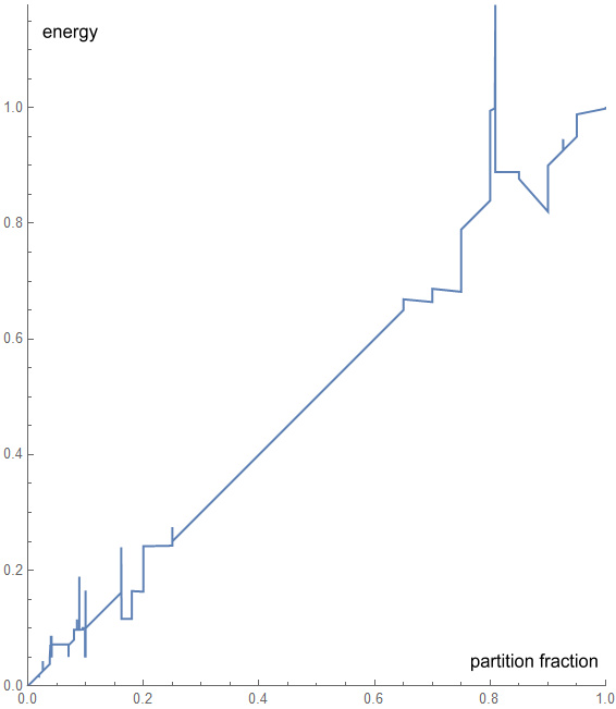
(Chart 1)

As can be seen, the line has sudden jumps.  These jumps occur at fixed positions of one hundred-thousandths of the overall width, i.e. in multiples of 0.00001.  And when the jumps occur, the energy will be in these same multiples.  To see the exact positions and values, open the accompanying app, view its source, and search for the array cvtspikengy

Over-unity notes

Of particular interest here is a section where the energy goes above 1.  I call these ‘over-unity notes’.  The highest over-unity note on the above chart occurs at fractional position 0.809 and has an energy value of 1.17772.  To hear what this sounds like, try comparing note 4.8378115541665725 with note 0.  The comparison reveals note 0 is more strongly base than normal.  For reference, a nearby note with energy of 1 is 4.838655592449876.

There are also over-unity notes of higher energy.  One of the highest found occurs at fractional position 0.41301409488.  It has an energy of 1.99989.  An example of this is note 4.836061673205495.  Comparing that to note 0 makes note 0 a very strong base.  These ‘super over-unity’ notes occur within very narrow regions – in this example, less than a trillionth of a semitone.

To hear some other examples, open the Sine Wave Piano app:

Sine Wave Piano

In the Temperament section are several tuning methods.  Start with the default Equal setting and alternate between notes C and E (using computer keys A and D).  In this setting, note E has an energy of 0.1069 and note C will sound as a weak base.

Next select the Stronger option and alternate between C and E.  In this setting, note E has an energy of 1, so note C will sound as a stronger base.

Next select the Over Unity+ option and alternate between C and E.  In this setting, note E has an energy of 1.99989, so note C will sound as a very strong base.

The Over Unity- option does the opposite and makes E the base.  But before playing other over-unity notes, either wait 29 seconds or change the Offset slightly, otherwise the notes will sound flat – see the following paragraphs.

There are several important points about how over-unity notes are affected by kill points.  The first is that both regular kill points and spike points will kill an over-unity note for four buffer lengths, i.e. for around 29 seconds.

The second is that over-unity notes will kill other over-unity notes for the same four buffer lengths.  That means if two such notes are playing within a 29 second period, some flattening will occur.

The third is that a long-duration spike point will kill an over-unity note for five buffer lengths, i.e. for around 35.7 seconds.

Measuring the energy

Determining the energy of a note can be done by comparing it to a note of known energy.

First select a partition that has spike points.  The widest runs from the kill point 4.834236543846192 to the peak 4.838655592449876.  Define Nx as a note between those two notes as follows:

Nx = 4.834236543846192*(1-x) + 4.838655592449876*x

Where x is a fractional position between the kill point and peak.  When x=0, it is at the kill point, and when x=1, it is at the peak.

Next choose a partition that has no spike points.  The widest with positive energy values runs backward from 4.867043954698947 to 4.866679973393758.  Define Ny as a note between those two notes as follows:

Ny = 4.867043954698947*(1-y) + 4.866679973393758*y

Where y is a fractional position between the kill point and peak.  Since this partition has no spike points, the value of y will also equal the energy of Ny.

Next choose a note that has note 0 as a strong base.  We can choose 5.82005 and call this note H.  H has an energy of 0.89.

To determine the energy of Nx, do the following:

Steps 6 and 7 should ideally be done using the ‘binary search’ method as that will quickly narrow down the target.

How do we measure the energy of a note when the energy is higher than 1?  This appears difficult because we don’t have any energies>1 in a non-spike partition.  The problem can be solved by noticing the energy comparison in the secondary buffer looks at the average of note energies.  So we also play note 0, which has energy of zero, and this halves the energy of the Nx note, as follows:

The result is that the energy of Nx is 2*y.

For example, if we set x=0.809, we will find y=0.58886.  This means the energy of Nx is 2*0.58886 = 1.17772.

Measuring the energy in reverse

An interesting thing happens when we reverse the above energy measuring process.  That is, instead of playing 12-Nx (a note from the spike partition) followed by 12-Ny (a note from the non-spike partition); we instead play 12-Ny then 12-Nx.

When we do it in this manner, instead of finding a single value where the two energies are equal, we instead find thousands of matching values.  The locations are best represented by this chart:

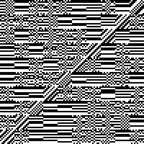
(Chart 2)

What we are seeing here is a tiny corner of a much larger chart.  The x-axis (along the bottom) represents the fractional positions within a spike-point partition, from 0.00000 to 0.00099.  I.e. the first 100 of 10,000 positions spaced at 0.00001.

The y-axis is likewise spaced at 0.00001 intervals and represents the energy measured in a non-spike-point partition.  When the ‘pixel’ at a given x/y coordinate is white, the energies are matched.  When it is black, they are mismatched.

This chart repeats itself 100 times along both axes.  That is, the first three digits of the five-digit fraction make no difference to the outcome.

There are many fascinating pattens here.  We can see a broader pattern of 10x10 large squares, represented by this table:

 S  H  S  S  S  H  H  S  H  D
 S  S  S  S  H  H  H  H  D  S
 S  H  S  S  S  S  H  D  H  H
 H  S  H  S  S  S  D  H  S  H
 H  H  S  H  S  D  S  H  S  S
 H  S  S  S  D  H  H  S  S  H
 S  H  H  D  S  S  S  H  H  S
 H  S  D  H  H  H  S  S  S  S
 S  D  H  H  H  S  S  S  S  H
 D  S  H  H  H  S  S  S  H  S

(Table 4)

Here, D contains diagonals, predominantly with white pixels on the locations where x=y.

H contains horizonal lines with each 1x10 column having the same pattern.

S contains ‘speckled’ patterns.

There are 5 S’s and 4 H’s in each row and column.

Within each 10x10 square, each column contains 5 white and 5 black pixels, with no more than 3 of the same type in sequence.  In the ‘speckled’ (S) squares, the 5th and 6th columns have a checkerboard pattern that is based on whether the S square has an even or odd horizonal location in Table 4.

The origin of these intricate patterns is unknown.  But it’s likely that they repeat themselves in some manner elsewhere in our hearing.