The Sideways Force

The preceding chapter on superconductivity proposed that electrons are able to move forever in a superconducting loop due to their receiving a small force in their direction of travel. As an electron passed a proton, field lines from the proton would pass through the electron at an angle. This caused the net force to be at an angle and a small component of it to run sideways to the proton.

I will call this component the Sideways Force and investigate its properties here. As it happens this force has many important implications beyond superconductivity.

Walking in the Rain

Previously we looked at this force as a result of field lines moving through a particle. Let’s now do it a bit differently. Suppose you were out walking one fine day and it suddenly started raining. You have a raincoat with you but forgot to bring an umbrella or hat.

Suppose the rain was falling vertically. If you stood still the rain would hit the top of your head. This would apply a vertical force to your head. You begin walking. As you do the rain starts to brush your face because you are now walking into some drops that fall in front of you. This creates a gentle backward force.

You walk faster. More rain now hits your face with greater velocity, increasing the backward force. Also the rain appears to be striking the top of your head at an angle, although its downward velocity hasn’t changed. You begin running. The rain strikes your face with even greater intensity. Meanwhile the force to your top seems to increase slightly. The overall force of the rain on your head has increased but has now shifted much of its intensity to your forehead and face.

What you are experiencing is a form of sideways force that comes about as a result of your forward motion through vertical rain. This is similar to the sideways force of the hunter’s bullet on the ducks. In this case the rain does not travel though your head; it bounces off it. But the net result is the same because your forward movement has changed the direction of force.

Calculating the Sideways Force on Charged Particles

Do field lines pass though charged particles (like bullets) or bounce off them (like rain)? My guess is that they pass through. However the question is unimportant for now since the result would be the same. So let’s just calculate what the resulting force strength and direction might be.

We’ll start with two electrons vertically aligned as shown:

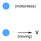
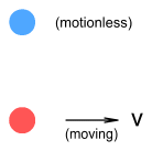
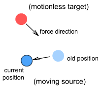
The top electron is motionless and the bottom one is moving to the right at velocity v. What will the force be on the top electron? In the chapter on Electric Fields I introduced the concept of field velocity, which is the velocity at which a field strikes a particle. Field velocity is a combination of light’s natural speed and the emitting particle’s movement.

The field leaves the bottom electron and travels upward at speed c. Meanwhile, due to the movement of the bottom electron, it is also moving to the right at velocity v. This produces a combination of right-angled velocities shown in the below diagram.

(Note: since velocity is purely relative it may be easier to imagine the bottom electron motionless and the top one moving to the left).

The above is a vector diagram so it will be easy to determine the net velocity using pythagoras:

$v_f = \sqrt{c^2+v^2}$

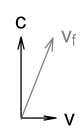
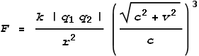
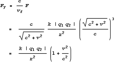
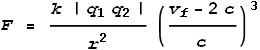
Where v_f is the field velocity, i.e. the speed at which the field hits the target particle (the top electron). We can now make use of the new equations given in the chapter on Electric Fields to calculate the force. These are like-charged particles so we use the push-field formula:

$F = \frac{k \left|q_1 q_2\right|}{r^2}\left(\frac{\sqrt{c^2+v^2}}{c}\right)^3$

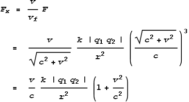
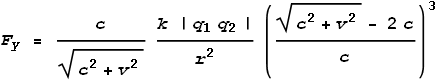
Where F is the net force. The direction of force will be upward and slightly to the right as shown in the vector diagram. We can now split this force into its x and y components by taking ratios of the component velocities:

$F_x = \frac{v}{v_f} F \text{ }= \frac{v}{\sqrt{c^2+v^2}}\frac{k \left|q_1 q_2\right|}{r^2}\left(\frac{\sqrt{c^2+v^2}}{c}\right)^3\text{ }= \frac{v}{c}\frac{k \left|q_1 q_2\right|}{r^2}\left(1+\frac{v^2}{c^2}\right)$

$F_y = \frac{c}{v_f} F\text{ }= \frac{c}{\sqrt{c^2+v^2}}\frac{k \left|q_1 q_2\right|}{r^2}\left(\frac{\sqrt{c^2+v^2}}{c}\right)^3\text{ }= \frac{k \left|q_1 q_2\right|}{r^2}\left(1+\frac{v^2}{c^2}\right)$

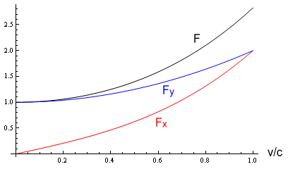
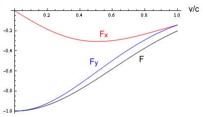
Now let’s see what that looks like on a chart. For simplicity we’ll set c=k=r=q₁=q₂ = 1. Here is the result:

The black line is the total force, blue is the y component and red is the x component. We see that as v increases, the x component, which is the ‘sideways force’, increases. Meanwhile the net force and vertical component (y) also increase but by lesser degrees.

The sideways force for opposite charges

What about the sideways force from opposite particles, such as the proton and electron below?

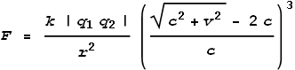
The electron at top is motionless and the proton underneath is moving to the right at velocity v. To determine the net force we again need to determine the field velocity. This calculation has already been done – it is the same as for the two electrons above. Field velocity is the same for all charge types. But the difference here is that we will use the pull-field formula [1]:

$F = \frac{k \left|q_1 q_2\right|}{r^2}\left(\frac{\sqrt{c^2+v^2}- 2 c}{c}\right)^3$

Next we’ll split this into x and y components by multiplying the net force F by the ratios of component velocities:

$F_x = \frac{v}{\sqrt{c^2+v^2}}\frac{k \left|q_1 q_2\right|}{r^2}\left(\frac{\sqrt{c^2+v^2}- 2c}{c}\right)^3$

$F_y = \frac{c}{\sqrt{c^2+v^2}}\frac{k \left|q_1 q_2\right|}{r^2}\left(\frac{\sqrt{c^2+v^2}- 2c}{c}\right)^3$

Here is the result on a chart:

The black line is the total force, blue is the y component and red is the x component. The lines are below the horizontal axis due to the forces being in opposite (negative) directions.

Here we see that situation is quite different between push and pull fields. For pull fields the net force and vertical component gradually decrease as v increases. Meanwhile the sideways force (the x component) is rather interesting. Its magnitude increases for a while and then levels out and starts dropping for large values of v. If the chart were extended to show v>c the forces would eventually become zero and then positive.

The sideways force at low velocities

The above charts show the sideways force at velocities up to light speed. In most situations however particle motion is confined to speeds within a few percent of light. Thus it is useful to understand the general properties of the sideways force at ‘normal’ speeds. Putting aside the unusual behavior at large velocities it can be observed that for small velocities and for both the push and pull fields we get:

$F_x \simeq \frac{v}{c} F$

$F_y \simeq F$

In other words, at low velocities (v<<c) the sideways force is directly proportional to velocity and the vertical force unchanged. For opposite charges it will be a promoting force (in the direction of a particle’s movement) and for like charges it will be retarding.

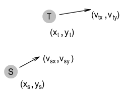
Generic equation for the sideways force

Let’s now develop a general purpose force equation that suits any arbitrary velocity and position.

The above diagram shows a Source and Target particle. Let the following terms be defined:

q_s = charge of source particle
q_t = charge of target particle
x_s = x coordinate of source	y_s = y coordinate of source
x_t = x coordinate of target	y_t = y coordinate of target
v_sx = x-component of velocity of source	v_sy = y-component of velocity of source
v_tx = x-component of velocity of target	v_ty = y-component of velocity of target

The formula for force components would be fairly complex if expressed entirely in these terms. So let’s break it down into its components.

First we’ll define distance terms:

$\text{$\Delta $x}=x_t-x_s$

$\text{$\Delta $y} = y_t-y_s$

$r=\sqrt{\text{$\Delta $x}^2+\text{$\Delta $y}^2}$

Where r is the distance between particles and Δx and Δy are the x and y components of distance.

Next we’ll define particle velocity terms:

$\text{$\Delta $v}_x=v_{\text{tx}}-v_{\text{sx} }$

$\text{$\Delta $v}_y=v_{\text{ty}}-v_{\text{sy}}$

Where Δv_x and Δv_y are the differences between velocities in the x and y directions respectively. Note that, for consistency with distances, they are in the form: target minus source.

Next we determine the field velocity. In a one-dimensional situation calculating field velocity would be a simple matter of adding source-particle velocity to the speed of light. In two dimensions however it is necessary to calculate the vector component of light speed in each of direction then add it to the source-particle velocity.

$v_{\text{fx}} = \frac{\text{$\Delta $x}}{r}c-\text{$\Delta $v}_x$

$v_{\text{fy}} = \frac{\text{$\Delta $y}}{r}c-\text{$\Delta $v}_y$

$v_f = \sqrt{v_{\text{fx}}{}^2+v_{\text{fy}}{}^2}$

Where v_f is the net field velocity and is calculated from the component velocities. Here you see that c has been multiplied by a ratio of distances to give its vector component. Particle velocity is then subtracted (instead of added) because the Δv terms represent the speed that the target particle is moving away from the source.

Now for the net force.

For push-fields (from like-charges) the net force will be:

$F = \frac{k \left|q_1 q_2\right|}{r^2} \left(\frac{v_f}{c}\right){}^3$

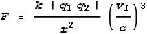
For pull-fields (from opposite-charges) the net force will be:

$F = \frac{k \left|q_1 q_2\right|}{r^2} \left(\frac{v_f-2 c}{c}\right){}^3$

From this the x and y components of force can be extracted:

$F_x = \frac{v_{\text{fx}}}{v_f} F$

$F_y = \frac{v_{\text{fy}}}{v_f} F$

That’s it! Using these equations we are now able to calculate electrical forces in any situation. These are for a two-dimensional situation but extending it to three dimensions is straight forward.

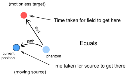
Phantom particles

Now for an important concept. In describing Coulomb’s Law we refer to the distance (r) between the source and target particles. From the view point of the target particle however, the distance from the source particle is actually irrelevant because the target particle reacts to the source particle’s field, not the source particle itself.

When a particle is moving it leaves behind a field pattern matching the at-the-time position and velocity; much the same way a ship leaves behind a ‘wake’. Since light has limited speed, this field takes a while to reach its target, by which time the source particle may no longer be at that position. Hence the target particle sees not what is but what was: it sees a time-delayed image of where the source particle used to be. The below diagram represents this:

I will call this old position of the particle a ‘phantom particle’. It represents a historical image of the source that is seen by the target. The position and velocity of the phantom is really what’s important in calculating the net force on the target. Determining the phantom’s position requires knowing how the source particle moved in the moments leading up to its current position. Here’s how:

The phantom’s position will be chosen such that the time taken for the phantom to reach the current position of the source particle equals the time taken for the phantom’s field to reach the target particle.

When the source particle is accelerating or moving along a non-straight path this calculation can be rather tricky. It’s also possible that more than one position could correspond to the phantom; although this would only apply to unusual situations (e.g. high accelerations or high velocities combined with sharp curvatures). In most situations however, we can ignore the tricky computations by assuming a constant-velocity and straight path. This will yield the generic sideways force equations shown above, and these are good approximations when v<<c.

So what is the best way to make calculations: consider the target motionless with the source moving, or the target moving with the source motionless? Strictly speaking we should consider the target motionless and use the position/velocity of the phantom particle as the source. In practice however, in low or constant velocity situations, it is easier to calculate by considering the source particle motionless.

Some other important aspects about the phantom particle:

1. The position of the phantom corresponds to a direct line-of-sight from where the force originates. If we know the phantom’s position we can ignore this ‘sideways’ concept and just say the force moves in a straight line from there.

2. The time taken for the field to travel from the phantom to the target can be used to determine the final field strength. This can be done by replacing the distance r with r = c T, where T is the time taken for the field to reach the target particle (or the time taken for the phantom to arrive at the current source position).

What we are saying here is that an electric field decays in proportion to the inverse square of its age. In other words time, rather than distance, is the determining factor of field strength.

Magnetism revisited

In the chapter on magnetism where we used the VDCL to calculate the amount of magnetic force based on current, an assumption was made that the force between charged particles will always be directly toward or away from each other. The above discussion on sideways forces however decrees this to not be the case. In view of this new information then, does this mean that those magnetic force calculations are invalid?

The answer is: no. As it happens, a computation, using the above sideways force formulas, of the magnetic force between two parallel wires of infinite length yields the same result. The computation will not be shown here as it is rather complex(!). But the important point is that this latest revision to the VDCL doesn’t violate the earlier predictions.

[1] Here we see the reason for having separate push and pull field formulas. If earlier versions of the VDCL were used the result would be different.