GPS Mythology – part 2

Secondary relativistic effects

The preceding chapter examined claims regarding the necessary application of Relativity to the Global Positioning System. It argued that, providing the satellites orbited at the same altitude and no adjustments were made to take Relativity into account, the largest error that could accumulate over a 24 hour period would be an unnoticeable 15cm.

This is nowhere near the enormous 11km that is frequently claimed. Take this quote from Relativity promoter Clifford Will for example:

“But at 38 microseconds per day, the relativistic offset in the rates of the satellite clocks is so large that, if left uncompensated, it would cause navigational errors that accumulate faster than 10 km per day! GPS accounts for relativity by electronically adjusting the rates of the satellite clocks, and by building mathematical corrections into the computer chips which solve for the user's location. Without the proper application of relativity, GPS would fail in its navigational functions within about 2 minutes.” [1]

Is he kidding? Nothing much is going to accumulate over a two minute period other than a miniscule error of 0.2mm. The only thing this paragraph demonstrates is that the majority of Relativity followers can’t think straight and function by blindly repeating the words of other followers.

Another problem we have is that the stated 38μs-per-day adjustments are made in the satellites rather than the receivers. The satellites are military equipment and contain special encryption used for accurate missile targeting. Hence a close examination of them would be off-limits to almost everyone including the majority of scientists. This makes the system somewhat inadequate as a test for Relativity. Even those who work at the GPS ground-monitoring stations with super-accurate clocks would be unable to determine what adjustments are made: Perhaps the satellites experience the stated amount of time dilation and adjustments. Or perhaps they experience different amounts of dilation and adjustments. Or perhaps they experience no dilation and no adjustments are made.

All that aside, some might argue that GPS can still be a good test of Relativity because there are a number of adjustments for ‘secondary relativistic effects’ built into the receivers that we can verify directly. The first has to do with imperfect orbits and the second with the Sagnac Effect. The purpose of this chapter will be to examine them, starting with the former.

Adjustments for eccentric orbits

In an ideal world, GPS satellites would be launched so as to sit in perfectly circular orbits at predetermined altitudes. In this way the amount of relativistic effect would be the same for every satellite and have a constant value throughout its orbit. Hence an identical timing adjustment could be programmed into each satellite to negate the effects. Such an adjustment would allow a GPS receiver not have to take relativity into account.

In the real world however, things don’t always proceed as planned. The satellites instead end up with slightly elliptical orbits. Because of this, the amount of time dilation will vary throughout an orbit as the satellites experience variations in their speeds and altitudes. And because of this, the fixed amount of relativistic adjustment that is built into satellites pre-launch is insufficient to negate the full effects of relativity. Instead, the receiver needs to make some of its own adjustments to get proper accuracy.

This May 2002 Physics Today article by Neil Ashby describes the situation:

“If a clock's orbit is not perfectly circular, gravitational and motional frequency shifts combine to give rise to the so-called eccentricity effect, a periodic shift of the clock’s rate with a period of almost 12 hours and an amplitude proportional to the orbit’s eccentricity. For an eccentricity as small as 1%, these effects integrate to produce a periodic variation of amplitude 28 ns in the elapsed time recorded by the satellite clock. If it is not taken properly into account, the eccentricity effect could cause an unacceptable periodic navigational error of more than 8 m.

During the early development of the GPS, onboard computers had limited capability. It was decided that correcting for the eccentricity effect would be left to the receivers. Inexpensive receivers accurate to no better than 100 m may not need to correct for the eccentricity effect. But, for the best positional accuracy, receiver software must apply a relativistic eccentricity correction to the time signals broadcast by each satellite. The navigation message includes the current eccentricity, orbital elements, and other information that the receiver needs for computing and applying the eccentricity correction.” [2]

The below diagram shows where these relativistic effects come into play.

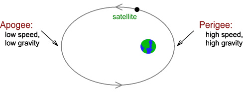
On the right side of the diagram is the perigee where the orbit is closest, and the left side is the apogee where it is farthest. (For visual ease the eccentricity is shown greatly exaggerated.)

The perigee has the highest speed and the lowest altitude. So it should have high amounts of both motion-based and gravitational-based time dilation.

The apogee has the lowest speed and the highest altitude. So it should have low amounts of motion-based and gravitational-based time dilation.

As a result, a clock in such an orbit would appear to run more slowly at the perigee and more quickly at the apogee. Because of this, receivers would need to make adjustments to the received clock signals in order to calculate position correctly.

Another explanation?

The fact that adjustments need to be made within the receivers would seem good evidence for relativity. Because, unlike satellite adjustments, what goes on inside the receiver can be easily confirmed – perhaps not by users, but easily enough by receiver manufacturers, of which there are many.

So does this mean the eccentric adjustments have confirmed relativity after all, or could there be another explanation?

In an earlier chapter on light it was proposed that light moves through a vacuum with a speed that is added to the speed of its source, i.e. at a speed c+v where v is the speed of the source toward the target. This is known as the “ballistic” or “emission model” of light.

Look again at the orbital diagram:

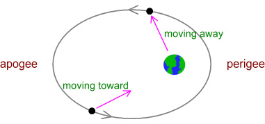
Note that as the satellite moves from the apogee to the perigee (farthest to nearest point), it is moving toward Earth. So a signal emitted during this phase would have the satellites’ speed added to it and move at speed c+v rather than just c. It would arrive sooner than “expected”.

Likewise as the satellite moves from the perigee to the apogee (nearest to farthest point), it is moving away from Earth. So a signal emitted during this phase would have the satellites’ speed subtracted from it and move at speed c-v rather than c. It would arrive later than “expected”.

Now if someone on Earth was under the assumption that the speed of the signal must always be c, they would likely be confused as they see the signals arriving earlier or later than their fixed-speed-of-light model predicted. They might conclude that the satellites’ clocks were somehow running at different speeds at different points in their orbit. So this person would be working under an erroneous assumption. And even though they would be able to use this assumption to accurately predict the arrival times of signals, their assumption would still be wrong.

Could it be then that this apparent periodic variation in clock rates is in fact just a change in the transmitted signal speed?

Ballistic model analogy

To answer this we need to look at a simpler analogy. Consider this classical mechanics situation:

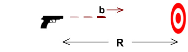
Here a gun aims at a target at distance R. The gun is motionless with respect to the target and fires a bullet at velocity b (relative to the gun). The bullet will take time T=R/b to reach the target.

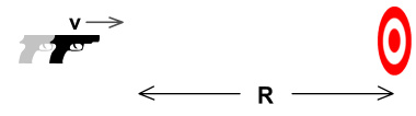
Now we change things a bit. In the above diagram, the gun moves toward the target at velocity v (relative to the target). When it is at distance R, it fires the bullet. How long will the bullet take to reach the target?

The bullet now moves at velocity b+v (relative to the target) because the gun’s velocity v is added to the bullet’s. Therefore it takes time T=R/(b+v).

The difference between these times is:

ΔT = R/b – R/(b+v) = R v/(b (b+v))

For values of v much less than b, i.e. when the bullet moves much faster than the gun, this closely approximates to:

ΔT ≈ R v/b²

Now translate the above to a satellite situation: replace the gun with a satellite and the bullet with a radio signal moving at speed c (relative to the satellite). Replacing b with c gives:

$\text{$\Delta $T} = \frac{R v}{c^2}$ (1)

This tells us that the signal will arrive earlier by a time difference proportional to distance and approaching velocity.

The calculated position error that would result from this time difference (if one were assuming light’s speed must be c) is determined by multiplying this by c. I.e.:

$\text{$\Delta $R} = \frac{R v}{c}$ (2)

So how would this translate to a real situation? Let’s say a GPS satellite had an eccentricity of 1%. The below graph shows its relative velocity toward Earth.

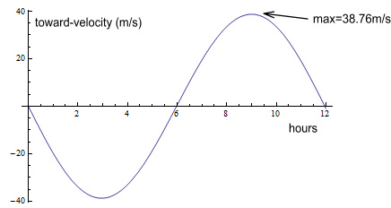
Here the horizontal scale represents time in hours over a 12 hour orbit. Hour zero is the perigee (closest) and hour 6 is the apogee (farthest). The vertical axis represents velocity toward the Earth. As can be seen, the velocity reaches a maximum of 38.76m/s on its approach and a minimum of negative the same amount on its departure.

This next chart shows the change in radial distance over the orbit:

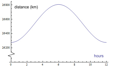
There is very little change, fluctuating by ±265km or 1% at most.

So what happens when we multiply these two charts in line with equation (2)? We get this:

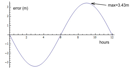
This shows the position error varies by plus and minus 3.43m. This is almost half the 8m described in the referenced article. In fact it turns out to be exactly half the relativity-calculated amount.

The GPS Navigation User Interface guide gives the exact equation that is to be used by receivers [3]. It is:

$\text{$\Delta $t} = -\frac{2 e\sqrt{G M A}}{c^2}\text{Sin}\left[E_k\right]$ (3)

This corresponds to the amount of cumulative time difference due to special and general relativity. e is the eccentricity, E_k is the “eccentric anomaly”, which is the angle of orbit measured from the centre of the ellipse, and G, M, and A are the gravitational constant, Earth’s mass, and satellite’s semi-major axis respectively.

So what would be the equivalent equation due to changes in signal speed? It works out to this:

$\text{$\Delta $t} = -\frac{e\sqrt{G M A}}{c^2}\text{Sin}\left[E_k\right]$ (4)

Comparing this equation with (3), we see it has the same form but it is exactly half the amount. Here is what a chart would look like comparing them for a 2% eccentricity (e=0.02) and multiplying by c to convert to position error.

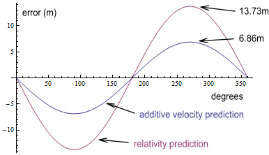
As can be seen, the prediction of relativity gives a maximum of 13.73m, while the prediction due to additive velocity gives a maximum of 6.86m. So it would seem that additive velocities can predict half the measured error. But since the receivers are programmed to accommodate for double that amount, does that mean the additive velocity idea is wrong and relativity is correct? Or is the other half adjusted for elsewhere? We’ll get back to that.

The Sagnac Effect

The other relativistic effect we apparently need to adjust for is the Sagnac effect. The literature explaining this is somewhat confusing so let’s ease into it with a couple of quotes:

The Physics Today article mentions:

“In the GPS, the Sagnac effect can produce discrepancies amounting to hundreds of nanoseconds. Observers in the nonrotating ECI inertial frame would not see a Sagnac effect. Instead, they would see that receivers are moving while a signal is propagating. Receivers at rest on Earth are moving quite rapidly (465 m/s at the equator) through the ECI frame. Correcting for the Sagnac effect in the Earth-fixed frame is equivalent to correcting for such receiver motion in the ECI frame.”

While Wikipedia says:

“GPS observation processing must also compensate for the Sagnac effect. The GPS time scale is defined in an inertial system but observations are processed in an Earth-centered, Earth-fixed (co-rotating) system, a system in which simultaneity is not uniquely defined. A coordinate transformation is thus applied to convert from the inertial system to the ECEF system. The resulting signal run time correction has opposite algebraic signs for satellites in the Eastern and Western celestial hemispheres. Ignoring this effect will produce an east-west error on the order of hundreds of nanoseconds, or tens of meters in position.” [4]

Based on this we can conclude that the Sagnac Effect:

has to do with the rotation of the Earth.
is most significant at the equator.
is very important to compensate for because it can
result in “tens of meters” of position error.

We will now investigate a more detailed source by the same author here [5].

On page 8 is a calculation discussing sending signals around the equator. It predicts a timing error of 207.4ns (equation 8). The calculation is rather complicated so let’s break it into easier steps:

If a signal was transmitted east along the equator it would take 0.1337 seconds to get back to its starting point (this could be done using mirrors or optic fibres for visible light, or re-transmitters for radio signals). Calculation: divide the circumference of the equator by the speed of light: 2*pi*6378137/(2.998x10⁸) = 0.13367s
But the equator is moving, and during that time the original transmission point would have moved east by 62m. Calculation: multiply that time by equatorial velocity: 0.13367*465.1 = 62.17m
It would take an additional 207.4ns to cover that distance. Calculation: divide that distance by the speed of light: 62.17/(2.998x10⁸) = 2.074x10^-7s = 207.4ns

At this point any rational person would have to be wondering: “What the heck does this have to do with the GPS?” GPS satellites don’t send signals around the equator!

When we read the words “Sagnac effect” it normally refers to light travelling around a circle via rotating mirrors, such as this typical laboratory-setup diagram shows:

Does this diagram resemble any portion of the GPS? Satellites transmit their signal to Earth and that’s that. There’s no transmission back to the satellites, or between satellites, and none of their signals are made to loop the equator. So in what way does the Sagnac effect have any relevance?

One place where the Sagnac effect would have relevance would be in the synching of ground-monitoring stations. There are six monitoring stations located roughly along the equator and these would need to be kept in-synch with each other. Such a process would need to adjust for the Sagnac effect, as the signal from the designated master station was transmitted to the others.

But the documentation discussing the effect insists that it is also relevant to GPS observers/users and that the receivers need to make adjustments for it or they will calculate “tens of meters” of position error. How to make sense of this, and what is the 207ns delay about?

Have a closer look at the motion of a satellite across the sky, this time including the shape of Earth:

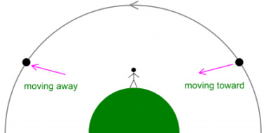
Here a satellite rises above the right horizon, passes directly overhead a user, and goes down over the left horizon. As it does so, notice that it spends time moving toward and away from the user. This graph shows the velocity in a straight-line direction, as viewed by the user:

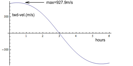
The velocity is zero when the satellite is directly overhead. But as it approaches, the toward-velocity goes up to 927.9m/s, when level with the horizon. And as it recedes, the velocity goes negative by the same amount.

Returning to our earlier discussion on additive velocities, this could mean the signal on the approach path arrives earlier than expected because net velocity is higher, i.e. c+v. Likewise it could take longer to arrive on the departing path because signal velocity is lower, at c-v.

Could this be the explanation for the timing differences? Satellites sit at an altitude of 20,184km. Plugging this into equation (1) gives:

ΔT = R v/c² = 20184000*927.9/(2.998x10⁸)² = 2.0837x10^-7s = 208.4ns (5)

This is quite amazing as we have arrived at an almost identical number as what the Sagnac-around-the-equator would predict! More importantly it was arrived at using very different inputs. The 207ns number used the equatorial circumference and velocity. Whereas this 208ns number used the satellite’s distance and velocity.

Could these additive velocities be the real cause of what is labelled “Sagnac effect”? It does seem more logical, especially as there is no reason why the Sagnac effect should have any relevance to the communication between satellites and receivers.

Near the end of page 9 is a discussion about an experiment done to measure the effect:

“In 1984 GPS satellites 3, 4, 6, and 8 were used in simultaneous common view between three pairs of earth timing centers, to accomplish closure in performing an around-the-world Sagnac experiment. ... The size of the Sagnac correction varied from 240 to 350 ns.”

“240 to 350ns”? Shouldn’t that be “0 to 207ns”? The effect is supposed to be due to Earth’s rotation, meaning it should be zero at the poles. And how did it get up to 350ns when 207.4ns represents the maximum possible (at the equator)?

Refer to equation (5). Here the distance used for R was the satellite altitude. This is only correct when the satellite is directly overhead. In reality the satellite-receiver distance will be larger when near the horizon. This graph shows the actual distance as the satellite moves overhead.

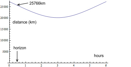
When level with the horizon, the distance is 25,766km. Using that value in equation (5) gives a timing value of 266ns (207.4ns will occur when the satellite is 29 degrees above the horizon).

This is above 240ns but still a fair way from 350ns. Perhaps that 350ns reading was done on an aeroplane and the satellite in question had an eccentric orbit. E.g. if the orbit eccentricity was 1%, this would increase the maximum R value to 26,800km. And if the aeroplane moved at 245m/s (a typical jet cruising speed [6]), we could add this to the 928m/s. Plugging this into equation (1) gives a value of 350ns. Now it is true that the reference didn’t say that one of the “timing centers” was on an aeroplane, or that they were all fixed on the ground for that matter. But how can they justify getting 350ns using the equatorial method?

We’ll look now at another reference here [7]. It appears to be a more detailed version of the previous reference [5]. On page 10 is a diagram that is reproduced below:

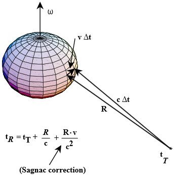
Notice there is a formula at bottom with the words “Sagnac correction” pointing to one of the terms. This term looks identical in form to equation (1), where R also refers to the distance between the satellite and receiver. This is quite a change from the previous reference where Sagnac corrections were calculated based on the Earth’s circumference.

The only difference between this and (1) is that v refers to the velocity of the Earth’s surface relative to its centre, rather than the velocity of the satellite relative to the surface. But should that be correct?

Taking the diagram at its word, the largest value of v will be the equatorial velocity of 465.1m/s. The largest R would occur when the satellite is on the horizon, which will be R=25769km. Plugging this into the suggested “Sagnac correction” gives:

v R/c² = 465.1*25769000/(2.998x10⁸)² = 133.3ns (6)

133.3ns? That is well short of the 207.4ns calculated using the “equatorial circumference” method. Something fishy is going on here!

On page 9 it gives the same equation (1.17) and equation 1.14 makes it clear that R refers to the distance between the satellite (r_T) and the receiver (r_R).

So what is v? In the paragraph above that it says:

“… and let the receiver have velocity v in the ECI frame.”

Where “ECI frame” means velocity relative to Earth’s centre, which corresponds to the velocity described in the above diagram.

Logically however, v should refer to the relative velocity between the satellite and receiver. After all, these are the components that make up the GPS. The velocity of the receiver relative to Earth’s centre should not be relevant, any more than the velocity of the receiver relative to Jupiter could be relevant. Earth just happens to be where the components are located. If we were to relocate the satellites and receivers to Mars, there is no reason why v should refer to Earth’s centre.

To understand this better, it would be helpful to refer to some specific calculations. To do this we can refer to the User Interface guide mentioned earlier [3]. Scanning this PDF for the word “sagnac”, we find no mention of the Sagnac effect!

Quite amazing. On one hand we are told that the Sagnac effect is important to adjust for otherwise it will result in “tens of metres of error”. But the interface guide gives no specifics on how to adjust for it, or even say that it needs to be adjusted for. It should be also pointed out that this manual is what GPS receiver manufactures are meant to rely on, so any necessary adjustments would have to be described there.

Does this mean the “Sagnac effect” (or additive velocity equivalent) adjustments have no relevance? I would say they do have relevance, but have been left out of the main guide and sent separately to manufacturers.

The reason for leaving out specific calculations might be to prevent researchers from seeing that the velocity v refers to the relative velocity between the satellite and receivers, rather than equatorial velocity. And the reason for not wanting people seeing this is that they might discover that the GPS shows that light’s speed is not a constant speed c, as seen by all observers, but varies with the speed of the source. Such a discovery would demolish the fundamental postulate of Special Relativity.

It appears there are other things left out of the manual. For example on page 113 a diagram says you need to compensate for “Tropospheric Adjustments”. However there is no mention in the guide about what adjustments to make (search the PDF for “tropospher”). But we can find plenty of information on the tropospheric adjustments elsewhere on the web e.g. by searching “gps tropospheric delay”. Searching the gps.gov website brings up 50 results over three pages [8].

By comparison, the only information available on the web for Sagnac adjustments for GPS appears to be copies of Ashby’s papers. Searching the gps.gov site for information on the Sagnac effect turns up only three ‘powerpoint’-type visuals [9]. These say the maximum is 133ns [10], which corresponds to equation (6). The absence of detail on the Sagnac effect on the gps.gov website is surprising to say the least!

Referring back to the Physics Today article [2], on page 46 is a column “Confusion and consternation”. It talks about the problem of adjusting for fast-moving receivers and says:

“One can estimate the discrepancies from the approximate synchronization correction: v x/c², where v is the receiver’s speed through the ECI frame and x is its distance from the GPS satellite in question.”

This looks similar to the “Sagnac” effect in equation (6). It then says:

“Within the framework of general relativity, however, one coordinate system should be as legitimate as another.”

That’s true, so why not make the receiver the reference frame and describe v as the relative velocity between satellite and receiver? It continues:

“Measurements made by an observer traveling with a moving receiver can just as well be described in another reference frame, by using transformations that relate the two frames. In the special case of two inertial frames in uniform relative motion, these are the familiar Lorentz transformations.”

This may be a clue. Transforming time using Lorentz transforms uses the formula:

$t' = \frac{t+\frac{v x}{c^2}}{\sqrt{1-(v/c)^2}}$ (7)

For values of v much less than c, the expression inside the square root becomes very close to unity. So this is approximately:

$t' \approx t+\frac{v x}{c^2}$ (8)

The expression on the right-hand side now looks like the additive-speed-of-light adjustment in (1). It’s possible that receivers manufacturers are told to make a Lorentz transform as shown by (7) and this effectively gives them an additive-speed-of-light adjustment.

It’s also possible that manufacturers are not given the specifics but need to figure it out themselves. The column begins with:

“Historically, there has been much confusion about properly accounting for relativistic effects. And it is almost impossible to discover how different manufacturers go about it!”

If the interface guide had given specifics for handling the Sagnac effect there should not be “much confusion” as manufacturers would go about it the same way. Perhaps manufacturers do their own experiments and end up settling with the Lorentz time transformation as shown in (7).

The TOPEX experiment

This brings us back to the earlier discussion about relativistic adjustments for orbital eccentricity. In order to resolve the question of reference frames, the Physics Today article goes on to discuss an experiment that tested for the eccentricity effects. It was done in space on a satellite called TOPEX. This diagram is provided:

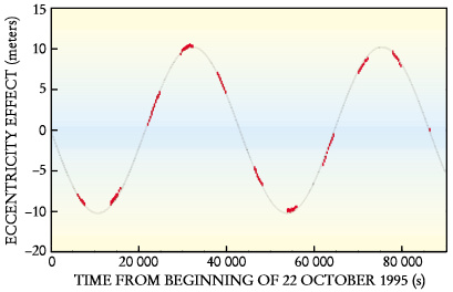
It shows the relativistic error for a GPS satellite with 1.5% eccentricity. For an eccentricity of 0.015, this calculates to a relativistic error of 10.3 metres, and this closely matches what is shown in the diagram.

An obvious question arises however – why do this experiment in space rather than on the ground? We have extremely accurate clocks in many laboratories. If it were possible to do it on the ground, then it could be verified independently. But if it were not possible, then we can’t know whether the eccentricity effect is due to relativity predictions or additive-speed of light predictions. Instead we must take the word of those promoting the relativity theory. This means the magnitude of the eccentricity effect is questionable, just like the existence of the 38.6μs-per-day adjustments.

Conclusions

There is no reason why GPS receivers should have to adjust for a Sagnac effect. Various ‘official’ calculations for the effect are inconsistent with each other. Whereas actual measurements don’t match the official calculations but instead correspond to an additive speed of light. Information on how to adjust for the Sagnac effect in receivers is strangely absent in the official user guide and gps.gov website.
The adjustment for orbital eccentricity is quite likely not a relativistic adjustment but an adjustment for a change in signal speed as the satellite moves toward and away from the receiver. The difference between the relativistic and the change-in-signal-speed predictions should be measurable on Earth but for some reason is done in space where it can’t be verified.

[1] http://physicscentral.com/explore/writers/will.cfm
[2] http://www.fing.edu.uy/if/cursos/fismod/GPS.pdf page 45 (pdf page 5), or here http://www.ipgp.fr/~tarantola/Files/Professional/GPS/Neil_Ashby_Relativity_GPS.pdf
[3] The user manuals are here: http://www.gps.gov/technical/icwg/ This is the most recent version: http://www.gps.gov/technical/icwg/IS-GPS-200H.pdf See page 96, or 109 on the PDF
[4] http://en.wikipedia.org/wiki/Error_analysis_for_the_Global_Positioning_System
[5] http://relativity.livingreviews.org/Articles/lrr-2003-1/download/lrr-2003-1Color.pdf pages 7-9
[6] http://hypertextbook.com/facts/2002/JobyJosekutty.shtml
[7] http://areeweb.polito.it/ricerca/relgrav/solciclos/ashby_d.pdf
[8] A search for "troposphere" on gps.gov
[9] A search for "sagnac" on gps.gov
[10] http://www.gps.gov/governance/advisory/meetings/2011-11/nelson.pdf page 14