Mercury’s Perihelion Advance

In 1846, famed astronomer Urbain Le Verrier embarked on a study of the planets in the outer solar system.  Uranus was the farthest known at the time and careful observation revealed its motion did not agree with the known gravitational influences of the other planets.  This led to the prediction and later discovery of Neptune.

Buoyed by this success, he turned his attention to the inner solar system and to a study of Mercury he’d started some years earlier.  Mercury was noted to have a strong elliptical orbit; at least in comparison to other planets.  It had also been noted that its orbit rotated as a whole, such that its closest point to the Sun –  the ‘perihelion’ – was seen to steadily advance over a period of years.  The reason for this was assumed to be that the outer planets’ gravity was pulling Mercury’s orbit around.

Le Verrier also assumed this but could not be sure if it were the entire reason.  By undertaking an onerous effort of detailed hand-calculations he determined that the outer planets should cause Mercury’s perihelion to advance by 527 arcseconds per century.  As part of the same exercise he determined its actual advance, based on observations spanning a century and a half, was 565 arcseconds/century.  This left a discrepancy of 38 arcs/century that could not be accounted for by Newtonian gravity.

A hunt then ensued to find out from where this 38 discrepancy might arise.  At first it was thought there might be an additional planet within Mercury’s orbit that was responsible.  Tentatively named ‘Vulcan’, this planet was searched for but never found.  Thereafter various modifications to Newtonian gravity were proposed to accommodate the discrepancy.

Using better observational data and improved calculations, the 38 discrepancy has since been revised to 43 arcs/century and the accepted explanation for it is that it is fully due to the predictions of General Relativity.  Wikipedia offers this table as a summary [1]:

Amount (arcsec/century)	Cause
531.63 ±0.69	Gravitational tugs of the other planets
0.0254	Oblateness of the Sun
42.98 ±0.04	General relativity
574.64 ±0.69	Total
574.10 ±0.65	Observed

Table 1: sources of the precession of perihelion for Mercury

There are two numbers of importance here.  One is the predicted amount advance due to Newtonian gravity, which is 532 arcs/cent.  The other is the observed amount of advance, which is 575 arcs/cent.  Now for something more important: if either of those numbers were wrong by a significant amount then the difference between them, 43, would also be wrong.  Unless that is, both numbers were wrong by the same amount and in the same direction.

Without access to the proper equipment it won’t be easy to challenge/analyse the observed 575 number.  But it will be possible to analyse the calculated 532 number, and that will be the focus of what follows.

The Ring-Planet Model

Le Verrier’s original analysis can be found here (in French) [2].  Since then a number of researchers have improved on his result using better observational data and calculation techniques.  They include: Le Verrier (repeat,1859), Newcomb (1895), Doolittle (1912), and Clemence (1947).  G. M. Celmence’s [3] is the ‘modern result’ quoted by Wikipedia in the above Table 1 (excluding his oblateness calc.).  Here is a comparison of their results:

Planet	Le Verrier	Newcomb	Doolittle	Clemence
Venus	276.312	277.649	276.188	277.881
Earth	90.747	91.433	90.700	90.038
Mars	2.471	2.485	2.472	2.536
Jupiter	152.900	154.004	152.904	153.584
Saturn	7.266	7.310	7.260	7.302
Uranus	0.141	0.141	0.141	0.141
Neptune	0.044	0.044	0.042	0.042
Total	529.881	533.066	529.707	531.524

Table 2: comparison of researcher’s results

An aspect these all have in common is that they model surrounding planets as though they were rings of uniform linear mass.  That is, they treat each planet as though its mass were evenly stretched along its orbit.  This diagram shows the idea:

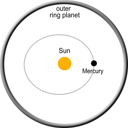
By doing this we can determine each ring-planet applies a net force on Mercury in a direction opposite the Sun and that this force will cause Mercury’s orbit to steadily rotate.  We can also calculate the contribution from each ring and sum them to get a total.

This reference [5] gives the basic method.  Equations (12) and (15) tell how to calculate the force and angular advance from a single planet.  By doing this for the planets we produce the following table (see the Mathematica notebook for the script that generated this table):

Planet	arcs/cent
Venus	268.871
Earth	93.532
Mars	2.387
Jupiter	160.093
Saturn	7.733
Uranus	0.145
Neptune	0.044
Total	532.805

Table 3: simple ring-model calculation

This table differs from Table 2 because we are modelling the planets as circles rather than ellipses and not adjusting for orbital elevations.  Still, it is very close, and this confirms that similar approximation methods were used by the people in Table 2.

Using Computer Simulations

Is this ring-planet method a valid model?  No doubt it is a convenient one because we only look at a planet’s average position and don’t have to worry about how an outer planet moves or that fact that gravity from a point source is different from a line source.  But convenience is no substitute for or guarantee of correctness.  A big problem that faces us is that modelling the influence from a planet’s actual position is going to be much harder to do – a ring-planet is difficult enough to model as it is.

No doubt some of the individuals listed above considered this problem but had no choice than to stay with the simplifications.  Luckily we in the modern age have a work-around: computer simulation.  By requesting a computer to consider the force/acceleration/ velocity/position situation at a point in time it can calculate an updated velocity/position at a small later point in time and repeat the process over and over.  No matter how complicated the forces involved, the computer simply chews through them and spits out accurate results.

So that is what we’ll be doing here.  Starting with simple situations to prove the concepts and then applying them to real data.  These simulations will be done using the software Mathematica.  For those who have access they can follow the steps and diagrams in this notebook:

download Mathematica notebook

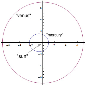
We’ll begin by considering a hypothetical solar system involving a ‘sun’, ‘mercury’, and ‘venus’ – spelt here in lower-case to distinguish them from the real bodies.

We’ll give this sun a mass of 50 units, mercury a mass of 1/100^th units, and venus a mass of 2 units.  Set the gravitational constant to G=1.  The sun will remain fixed at position (x,y)=(0,0), mercury will start at (1,0) and venus at (7,0).  mercury will have an eccentricity of 0.4 and venus will move in a perfectly circular orbit, i.e. with an eccentricity of zero.  This diagram shows how both planets would move if neither influenced the other:

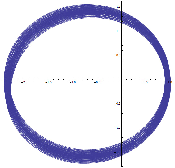
Now allow mercury to be gravitationally influenced by venus, but the sun’s location and venus’ orbit will remain unchanged.  This is the result after 200 seconds:

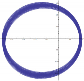
(click to enlarge)

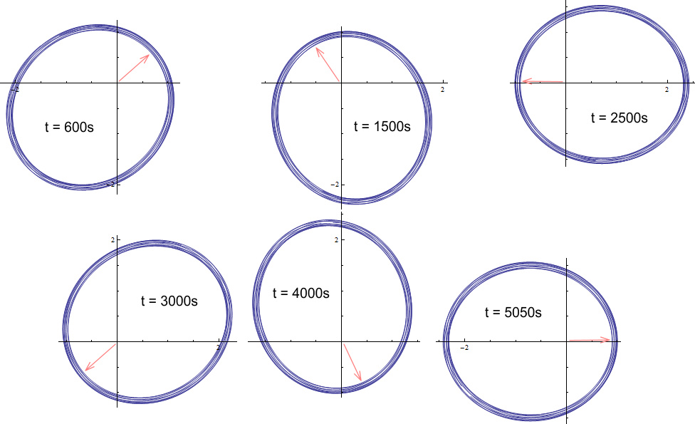
We now see mercury’s orbit wobbling and being dragged forward by venus.   If we allow the simulation to continue, this is how mercury’s orbit would look during selected periods:

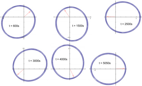
(click to enlarge)

It appears to take 5050 seconds for the ellipse to fully rotate.  That corresponds to 360/5050 = 0.071 degrees per second, or 4.28 degrees per minute.

Instead of displaying the results this way we could instead just plot the angle of perihelion point as a function of time.  Doing this over a 10 minute period shows:

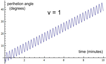
Here we see the perihelion point oscillate back and forth somewhat but overall it moved forward about 42 degrees.  A line-of-best-fit to this graph reveals a gradient of 4.28 degrees per minute, which agrees with the above.

Now redo the simulation.  Everything will be kept the same except that venus will orbit with exactly double the velocity.  This is what a chart of the perihelion angle shows:

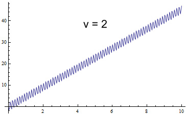
As might be expected, the oscillations have double the frequency because venus is passing mercury twice as often.  They are also of lower magnitude.  But the more interesting point is that the slope is steeper, reaching 44 degrees.  The actual slope is 4.53 degrees per minute.  So increasing the velocity increased the perihelion advance.

Now redo it with venus moving at half the original speed:

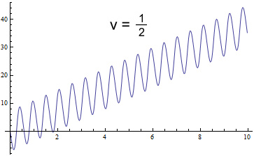
The oscillations are slower and broader and the slope is reduced to 3.86 deg/min.  By slowing the velocity we have reduced the amount of perihelion advance.

The next result is even more interesting.  We will reduce the speed to one tenth (1/10^th) of the original:

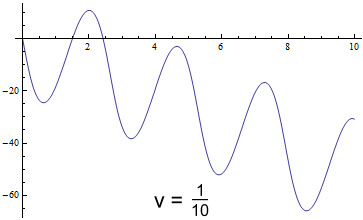
The perihelion is no longer advancing but receding!  The slope on this is minus 5.20 deg/min.  Further experimenting shows that making the velocity 0.155 times the original yields a flat slope, with mercury wobbling but making no overall progress.

As a final example we’ll make venus orbit in the opposite direction with the exact negative of the original velocity:

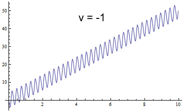
Rather than push the perihelion backward, it is causing it advance faster, with a slope of 5.01 deg/min.  Some might object to this example because outer planets don’t orbit backward.  But according to ring-planet model it should make no difference what the direction was.

What the above reveals is that the ring-planet model is not a valid method of calculating perihelion advance and that we must also take into account the speed of the orbiting planets.  It was not easy for people living decades ago to know this.  But with modern computers, anyone can confirm it easily.

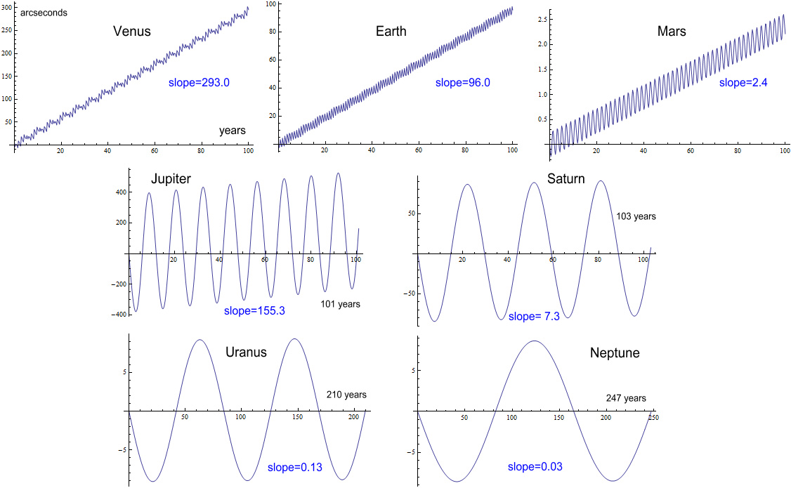
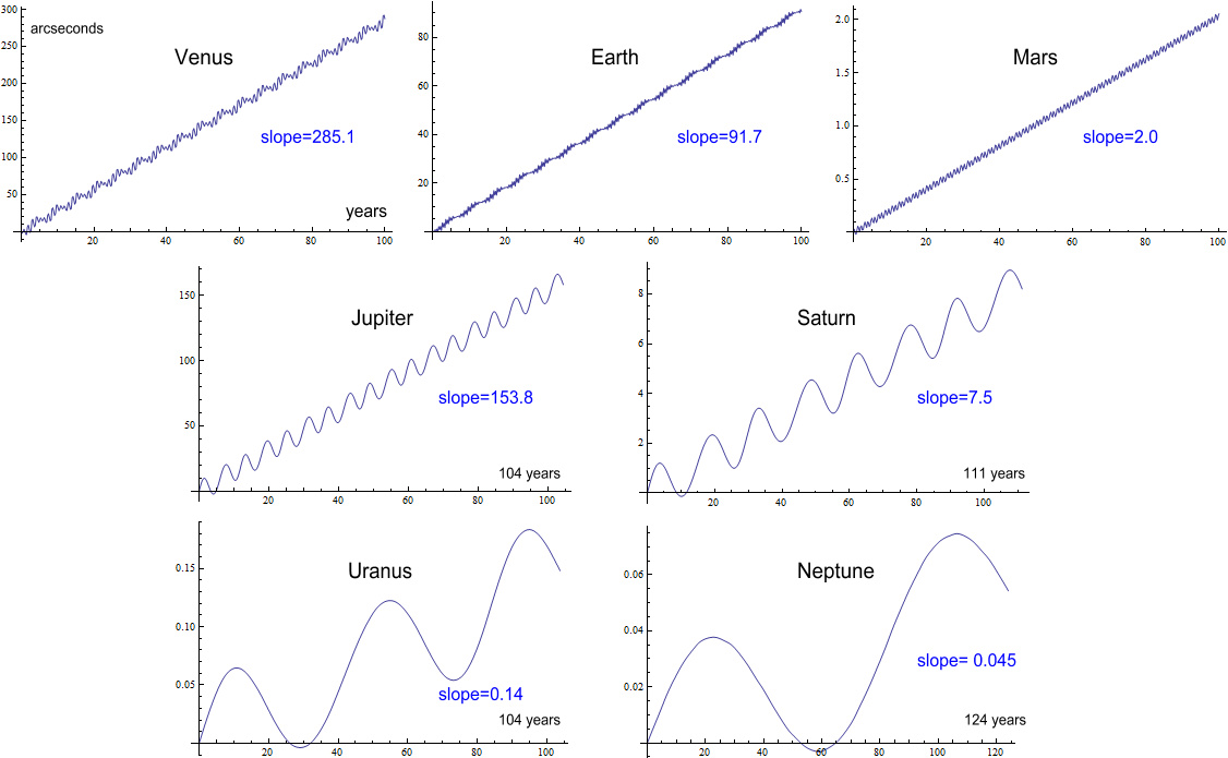
Having done this, we will now apply the above method to real data.  Doing this for each of the outer planets from Venus to Neptune over a hundred year period (or more for the outer planets) yields the following charts:

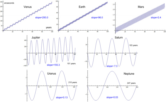
(click to enlarge)

This gives the following table:

Planet	arcs/cent
Venus	293.0
Earth	96.0
Mars	2.4
Jupiter	155.3
Saturn	7.2
Uranus	0.13
Neptune	0.03
Total	554.1

Table 4: contributions from a fixed Sun

Comparing this with Table 2 shows the results to be similar for most planets.  Venus and Earth give a notably higher contribution of an additional 15 and 6 arcs respectively.

The overall total is 554 arcs/cent.  This is very different from the ‘official’ total of 532 arcs/cent.  But we are far from done because there are many other aspects to consider.

Contributions from Multiple Planets

Another assumption made by the ring-planet model is that it is acceptable to calculate the contributions from surrounding planets individually and then total them.  This might seem reasonable because Newtonian gravity is additive, so presumably perihelion advances should likewise add.

To find out if they do, we will add a second orbiting planet to our hypothetical system.  Call this ‘jupiter’, give it a mass of 4 units and start it at (14,0), i.e. at double the venus distance.  Its orbit will be perfectly circular and its velocity will be smaller than venus’ by the square-root of 2 (since that’s what orbital mechanics requires).  Removing venus from the system, and plotting jupiter’s contribution on mercury’s perihelion shows the following:

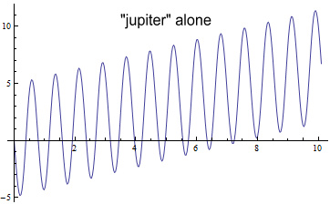
The slope of this is 0.65 deg/min.

Now redo the simulation with both venus and jupiter acting on mercury simultaneously.  Here’s the result:

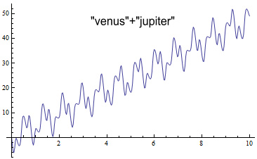
The wobbles in the perihelion angle have become rather complicated because it contains a high-frequency contribution from venus and a low-frequency from jupiter.  The average slope of this is 4.78 deg/min.

Recall that venus on its own causes a slope of 4.28 and jupiter causes 0.65.  Adding 4.28+0.65 gives 4.93.  This is greater than the 4.78 contribution from both planets when acting together.

What this shows is that we can’t simply add contributions from individual planets and expect a sensible total.  Instead we must consider the planetary effects all at the same time.  Doing this algebraically on paper will be next to impossible.  But with computers… no problem at all.

So now to try this with real data.  Rather than doing all the planets at once, we’ll start with Jupiter and Saturn since they have the largest combined influence.  Doing so gives this chart:

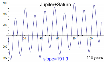
The chart contains a main wobble from Jupiter and a lesser one from Saturn.  The slope of this chart is 192 arcs/cent.  Adding together the stand-alone contributions from Jupiter and Saturn would predict 155+7= 162.  So their combined contribution is greater than their sum by 30 arcs.

Now to simulate the contributions of all planets from Venus to Neptune.  Here’s the result:

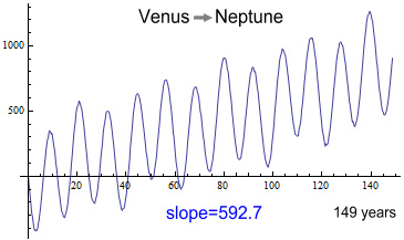
The chart is now very wobbly as it contains contributions from seven planets, although most are too small to see.

The overall slope is 593 arcs/cent.  Whereas the sum of their individual contributions was 552 arcs/cent.

That’s an increase of 41 arcs and the result is now larger than the observed 575 number.  This also shows the ring-planet model is rather busted, and yet there is still more to consider.

Motion of the Sun

When modelling the solar system it is common practice to consider the Sun fixed at a central point while the other planets orbit it.  But in reality the Sun moves about quite a bit, due mainly the influence of Jupiter and Saturn.  This diagram shows a sample of its motion:

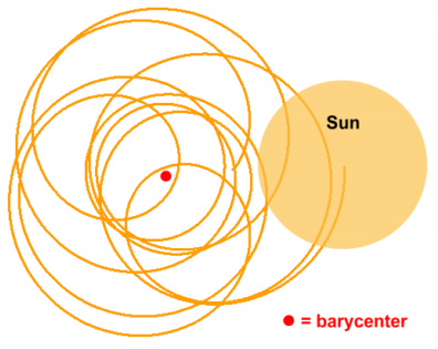
Motion of the Sun around the Solar System Barycenter.  (source: orbitsimulator.com)

The Sun will often move outside of its average location by over a full radius.  For some reason this never appears to be considered when modelling Mercury’s perihelion motion.  Table 1 mentions the influence from the Sun’s oblateness, which is the bulge at its equator.  This oblateness is a mere one part in a hundred thousand and is considered in Mercury’s motion.  Whereas a movement over 100,000 times the bulge is completely ignored!

Given the complexity of motion, the fact that it was ignored is understandable, but certainly not excusable.  It would have been better for the earlier researchers to admit that the problem was unsolvable rather than claim to have a definitive answer (and end up misleading everyone).

So how then would the Sun’s motion affect Mercury?  To answer this we will return to the simple simulation of the ‘sun/venus/mercury’ system but this time allow the sun to move freely.

Allowing the sun to move means that venus will be instead orbiting a barycentre, which will be the centre of mass for this system.  This will require giving venus a slight boost in velocity in order for it to have a circular orbit.  Doing this results in this perihelion advance:

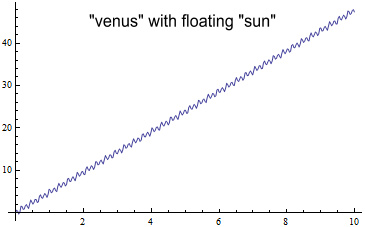
The first thing that stands out is that allowing the sun to move freely results in much less wobble for the overall orbit and perihelion.  Actually the orbit is wobbling quite a bit when viewed relative to the system’s barycentre.  What is shown here is the motion of mercury relative to the sun, because that is how the real Mercury’s orbit is measured.

The slope of this line is 4.78deg/min.  This is larger than the 4.28deg/min when the sun was fixed.   If we give venus the same starting velocity as before (when the sun was fixed), its orbit will be slightly elliptical rather than circular, and mercury’s perihelion slope will be 5.68deg/min.

What this shows is that there is a distinct difference between having the Sun fixed vs. free-floating.

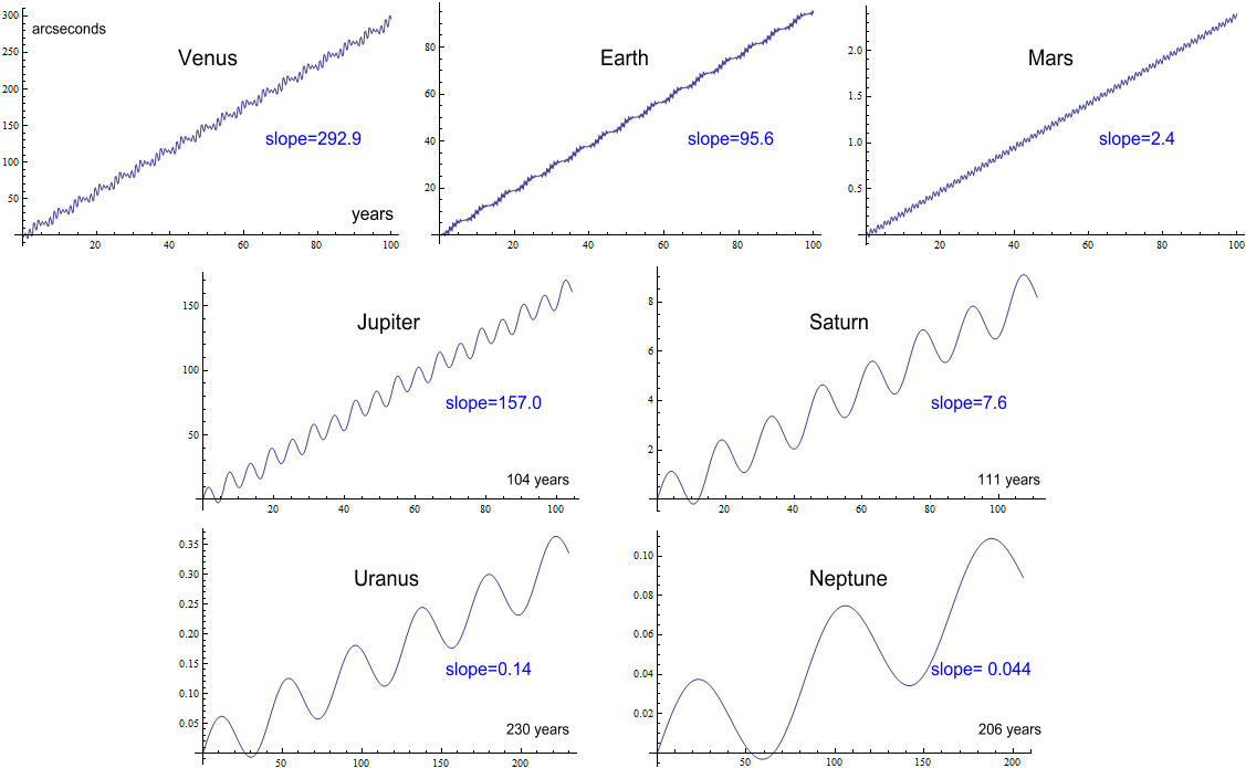
We’ll now apply the same simulation to the actual planets.  The starting velocity of each outer planet will be given a slight boost in order to make its orbit period match the observed.  Here are the charts:

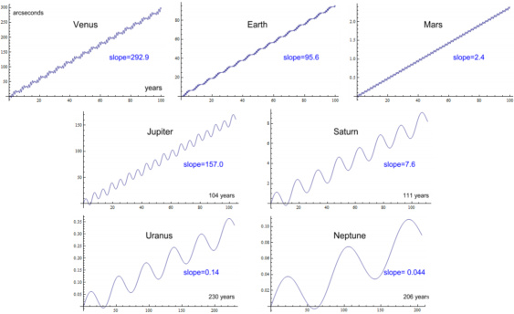
(click to enlarge)

Planet	arcs/cent
Venus	292.9
Earth	95.9
Mars	2.4
Jupiter	157.0
Saturn	7.6
Uranus	0.14
Neptune	0.04
Total	556.0

Table 5: contributions from a floating Sun

Comparing this with Table 4, the perihelion advances have decreased for the inner planets and increased for the outer planets.  The overall total is 556 – an additional 2 arcs.

So the effects of a floating Sun turns out to be not much different from the fixed Sun situation, but still substantially more than the effects of oblateness (0.0254arcs), meaning that the motion of the Sun shouldn’t be ignored.

Eccentric Orbits

Up until now the planets surrounding Mercury have been modelled as having circular orbits.  In reality their orbits are slightly elliptic or ‘eccentric’.  So we need to redo the above using the proper orbit shapes.  Doing so gives these charts:

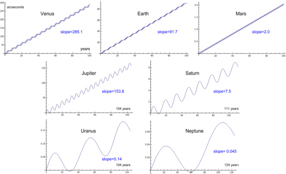
(click to enlarge)

Planet	arcs/cent
Venus	285.1
Earth	91.7
Mars	2.0
Jupiter	153.8
Saturn	7.5
Uranus	0.14
Neptune	0.04
Total	540.3

Table 6: contributions from eccentric orbits and a floating Sun

Comparing this to Table 5 shows the effects have been reduced and the total is 16 arcs less at 540 arcs/cent.

The next step is to combine these eccentric orbits so that they are happening simultaneously.  Doing so gives:

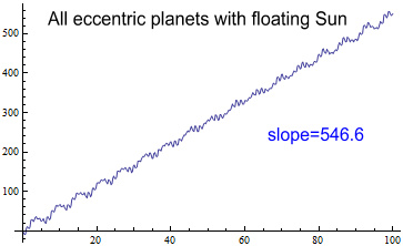
The result is 547 arcs/cent – 6 more than when the effects were applied separately.

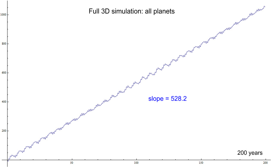
Putting it All Together

There is a final important aspect to consider, and that is the fact that the planets don’t orbit in the same plane.  Instead, each planet, including Mercury, is a tilted ellipse, and their perihelions don’t line up either.

To find out what the effect of all this is will require a full three-dimensional simulation of the Solar System, with each of the planets’ orbits set at their proper inclination, tilt and rotation.  Doing this over a period of 200 years gives the result:

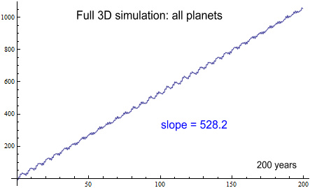
(Fig. 20 - click to enlarge)

The slope on this is 528.2 arcs/century.  Comparing this with Table 1 shows that this is 3.4 arcs less than the 531.6 arcs calculated using the ring-planet model.

Adding in 0.025 arcs for solar oblateness brings this simulated number up to 528.25 arcs.  This means the discrepancy between the observed and simulated calculated is 45.85 arcs, which is 2.9 arcs or 6.7% higher than the General Relativity prediction of 42.98 arcs.

Is this 3 arcseconds discrepancy a problem?  According to Table 1, the error in the observed value has an error of +/-0.65, so 3 arcs is well outside the maximum error.  The above chart (Fig. 20) was simulated with an accuracy of 10cm over 200years and so should be quite reliable.

We can redo the simulation using the aphelion as the starting point for the outside planets, with mercury still starting at its perihelion.  Doing so gives a very similar result of 528.3 – see chart here.   This shows that the starting location of the outside planets is not important to the long-range average.

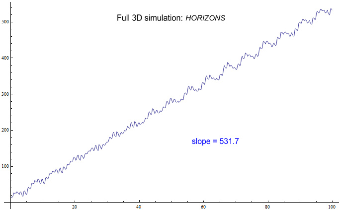
Using HORIZONS Data

There is another source of data we can use to get starting positions and velocities for all the planets and the Sun: JPL’s HORIZONS system [6].  It can give us the position and velocity of all the planets the Sun for a requested date and time, relative to the Solar System Barycentre.

The starting time will be chosen as February 1^st 2001 at 15:14, because this corresponds to a perihelion point of Mercury.  With these starting conditions, running a simulation over a hundred year period gives this result:

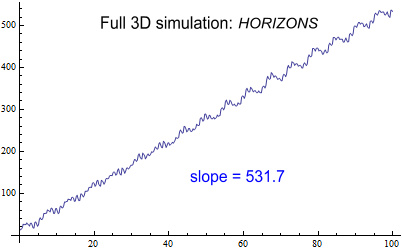
(click to enlarge)

The slope on this is 531.7 arcs/century.  This is now almost identical to the ‘official’ amount of 531.63 arcs/century.

What has happened?  Why does this not agree with the above simulation showing 528.2 arcs?

A casual look at the end positions of the planets shows Earth to be in a very different location than where it started – 22 degrees further ahead.  After 100 years, or any integer multiple number of years, Earth should be at the same place as where it started.

Looking at the other planets and comparing their simulated location to where HORIZONS says they should be located 100 years later (February 2^nd 2101 at 15:14), shows they are also far removed from where they should be.  How could that be when the simulation accuracy was set so high as to be only out by 10cm?

Further investigation revealed this was because the simulated orbit periods were too short.  Earth should have an orbital period of 365.26 days, but the simulation showed 365.03 days.  Over a hundred year period Earth thus lost 23 days and ended up 22 degrees further ahead in its orbit.

Similar problems were evident with all the planets – all except Neptune had too short an orbit period.  This table reveals the extent of the problem:

Planet	period (should be)	period (calc)	error %	degree error after 100 yrs
Mercury	87.97	87.908	-0.07	105.4
Venus	224.7	224.587	-0.05	29.4
Earth	365.26	365.031	-0.06	22.6
Mars	686.98	686.66	-0.04	8.9
Jupiter	4332.82	4329.86	-0.06	2.1
Saturn	10755.7	10747.44	-0.07	0.9
Uranus	30687.2	30668.05	-0.06	0.3
Neptune	60190.0	60198.08	+0.01	-0.03

Table 7: errors in orbital periods from HORIZONS data

The majority of planets have an orbit period around 0.06% less than they should have.  For the inner planets this leads them being in completely the wrong location.  Mercury is ahead by 105 degrees!

By comparison the simulation used on Fig. 20 was out by 6.3 degrees for Mercury and 0.5 degrees for Earth (over a 100 year period).

Looking further into the cause of this reveals that HORIZONS is giving us the correct positions but wrong velocities of the planets.  The velocities are being understated and this results in planets orbiting closer to the Sun with shorter periods.

For example at Mercury’s perihelion, to get a period of 87.97 days, the tangential velocity needs to be 58,987m/s.  Instead it is 58,977m/s – 10m/s less – and this results in a period of 87.908 days.  For Earth, the velocity at perihelion needs to be 30,292m/s.  But HORIZONS (at 2001-01-04 08:53) says it is 30,282m/s, giving a period of 364.90 days.

So the velocities are wrong, and they lead to orbits closer to Mercury and a larger perihelion advance.  Given that this advance is almost identical to the amount required by GR, there’s a strong possibility that the velocities have been deliberately tampered with in order to confirm the predictions of GR.

Conclusion

Early analysis of Mercury’s motion was based on simplified models that ignored aspects such as the outer planets’ speeds, their combined contributions, and the motion of the Sun.  This led to the conclusion that Newtonian gravity would predict Mercury to precess by 532 arcseconds per century, and that there exists a discrepancy of 43 arcs/cent that can be attributed to General Relativity.

A proper analysis that considers all aspects of Solar System motion however shows the Newtonian prediction to be 528 arcs/cent, making the discrepancy 46 arcs/cent, and this is not in agreement with GR.

[1]  https://en.wikipedia.org/wiki/Tests_of_general_relativity
[2]  http://articles.adsabs.harvard.edu//full/1859AnPar...5....1L/0000008.000.html To read in PDF form, click on the ‘Print this article’ (top right), click on the ‘YES’, and that will open/save as a single PDF.
[3]  http://journals.aps.org/rmp/abstract/10.1103/RevModPhys.19.361  A backup copy is here.
[4]  http://www.jstor.org/stable/10.2307/1005431
[5]  http://www.math.toronto.edu/~colliand/426_03/Papers03/C_Pollock.pdf
[6]  http://ssd.jpl.nasa.gov/?horizons
  Select ‘Web Interface’, then apply these settings:
     Ephemeris Type:  VECTORS
     Target Body:  Mercury [199]
     Coordinate Origin:  Solar System Barycenter (SSB) [500@0]
     Time Span:  Start=2001-02-01 15:14, Stop=2001-02-01 15:15, Step=1 m
     Table Settings:  output units=KM-S; quantities code=2
     Display/Output:  default (formatted HTML)
   Then click ‘Generate Ephemeris’.  The starting position/velocity of Mercury will be the X/Y/Z and VX/VY/VZ of the first entry (15:14:00), multiplying by 1000 to convert to metres.  Then repeat this for each of the planets, including the Sun, by changing the ‘Target Body’.