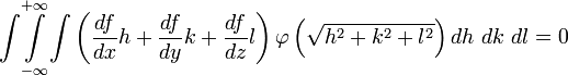
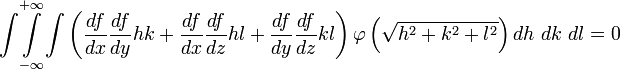
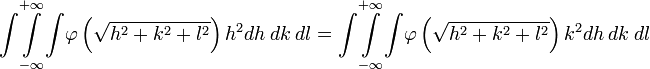
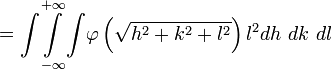
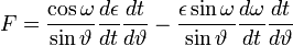
The Spatial and Temporal Propagation of Gravityby 1. The Basic Law.Gravitational phenomena are the only effects concerning separate bodies for which we cannot prove that the intervening space has a role, i.e. the existence of changes that are communicated through it from one place to another. All the more understandable therefore is the hope that we will ultimately succeed in finding the missing evidence. However we must not regard the matter as if there was no doubt that this exception was only an appearance. All known and understood observations strongly suggest the opposite. Therefore, if this is still only based on a lack of empirical information or incomplete analysis, it must first be demonstrated that there are facts that rectify and complete our previous conception in the opposite sense. Therefore it is necessary above all to exclude any hypothesis that assumes that some event occurs in the space between two gravitating masses that is responsible for gravity. Reference was made to previous similar, but inadequate treatment of the issue discussed here, in the report made by Drude on remote effects in the 69th Naturforscherversammlung (Natural Scientists Meeting). Two gravitating masses can be recognized as such by the resistance by which they oppose an enlargement of their distance. There must therefore, while the masses themselves can be at rest or in motion, be a connection between some of the events existing in the space between them. Obviously, with the position, or with the position and the current state of motion of the masses, insofar as external influences are excluded, we mean not just the resistance from one point of mass, but also the infinite sum of resistances from all other points of mass. The necessary work to overcome the resistance is therefore the same as the single resistance of a strength characterized by that of gravity. Whether changes that propagate in space with loss of time are linked with gravity or not, it can merely, where it matters, be considered as being a parameter. For there is no sense in speaking of the concept in terms of the spatial propagation of the resistance or the attraction, because resistance and attraction exist as such only in the places where the masses are located. But if it is predicated that an event requires time to communicate from one place to another, then this means the event cannot be existing at one place while simultaneously existing at another; it must cease to exist at the first point before existing at the second. In this way the energy contained in the event would decrease with time, if it did not pass through only those points lying directly between the two places, but through other points also. The energy is equal to the work required to communicate the event, as it pertains to gravity, between two masses located in different places. This energy then depends on the position and the momentary state of motion and these cannot induce two different levels of energy. Now in order to differentiate let us call one mass the attracting and the other the attracted. Let V be the potential of the attracting mass on the attracted. Let Vm be the amount of work required to be performed on the attracted mass to separate it from the attracting mass to an infinite distance. Let the coordinates of the point at which the imaginary mass m is being held, with reference to the likewise held attracting mass, be x, y and z. One can calculate V using the methods described in Mach’s principles of thermodynamics, by equating it with the mean of all the prevailing potentials in the immediate neighborhood of the point. V is of course not a vectored quantity and for a given location is constant with time. Let m be experiencing a force equal to f (x, y, z) and for a neighboring point equal to Furthermore, let  represent the density of the mass m (at point x+h,y+k,z+l) and which as an effect depending on proximity decreases rapidly with increasing distance. Then we find 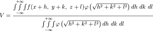 Expanding f as a Taylor series to the second power, and integrating over the point x, y, z, this becomes
Then by setting 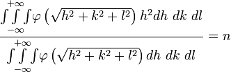 sets, 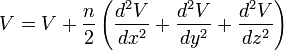 , ,So that 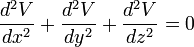 . .From this equation it follows in the well-known way, if µ is a constant and r means the distance of the masses,  . .This amounts to Newton’s law of gravity. Because 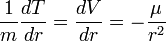 . .Newton's law defines the potentials that reach the masses in every position if they have the necessary time to achieve their realization. This condition is always satisfied when the masses are held at a distance from each other. The condition ceases in the case of free movement directed towards each other, if the time concerned has a finite measured size. Two factors are of importance. First, the potential must indeed begin to form at a distance r - Δr of the masses, where Δr is positive when r increases and negative when it decreases, to achieve stationary size in the inverse proportion of r - Δr, because it would otherwise not be possible to see how this relationship could be fulfilled when the masses are at rest. But the effect is not immediately imposed on m, because the conditional process starts from the attracting mass and needs time in order to proceed to the attracted mass. Of course, the same kind of progression also occurs from the attracted to the attracting mass, similar to the counter-radiation occurring to any radiation of heat between two bodies. The outbound potential at the distance r - Δr of the attracting mass manifests itself therefore in m only at a later time Δt, after the distance has become equal to r. Second, the potential as a long-distance effect would indeed appear immediately in its full amount; however, time and space are to be taken into account in the assumed way, so a certain duration of time is also necessary, so that, once arriving at m, this mass influences, i.e. causes the corresponding state of movement of m. For only the assumption of remote effects allows for discontinuity in the phenomena; its replacement by the assumption of effects of close proximity primarily has the purpose of introducing the continuity which has been demonstrated in other physical and chemical changes in the understanding of gravity. As therefore with an impact the momentum of the impact is composed of successive elementary impacts, the transmission of the event that is the arrival of the potential on m happens by fast successive differential potentials. If the masses are at rest, the movement of the potential to m happens at its own pace; then the value transferred on m is defined by the inverse proportion to the distances. When the masses are hastening towards each other, the time of the transfer is reduced, and thus also the value of the potential transferred in proportion of the speed of the potential itself to the sum of this speed and the speed of the mass, since the potential has this overall speed in relation to m. Apart from its speed c, the potential also moves with the speed of the attracting mass, from which it emanates. The path r - Δr, which the two approaching movements, that of the potential and that of the attracted mass, travel in time Δt, amounts therefore to 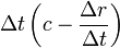 ; ;while r = c Δt. So we obtain for the distance at which the potential begins to form, and to which it is inversely proportional 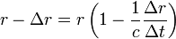 . .Because furthermore the speed with which the movements are approaching each other has the value  the potential drops due to the time needed before its effect on m, which is also proportional to  We therefore find 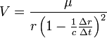 . .As long as the route Δr is short and therefore 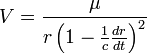 , ,whence with the aid of the Binomial theorem to the second power, we get ![V=\frac{\mu}{r}\left[1+\frac{2}{c}\frac{dr}{dt}+\frac{3}{c^{2}}\left(\frac{dr}{dt}\right)^{2}\right]](img/PG1-eqn20.png) . .The expression for V contains not only r, but also the derivative of r with respect to time. Therefore, by virtue of general Lagrange equations of motion, this gives the acceleration of m, when ![\frac{1}{m}\frac{dT}{dr}=-\frac{1}{m}\frac{d}{dt}\frac{dT}{dr'}=\frac{dV}{dr}-\frac{d}{dt}\frac{dV}{dr'}=-\frac{\mu}{r^{2}}\left[1-\frac{3}{c^{2}}\left(\frac{dr}{dt}\right)^{2}+\frac{6r}{c^{2}}\frac{d^{2}r}{dt^{2}}\right]](img/PG1-eqn21.png) . .The assumption that 2. The speed of propagation.According to whether the observations provide a finite or an infinite value for the quantity c introduced in the previous calculation, one finds more or less certain that the potentials of gravitating masses need time to traverse the distances lying between them, or that such temporal propagation does not exist, and thus the gravity is based on true distance. In particular, it requires the fulfillment of two requirements. First, due to the great magnitude of c over We state 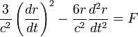 . .So we then have
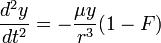
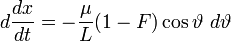
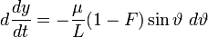
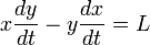
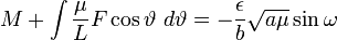
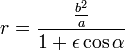
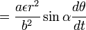
whence, by multiplying one equation by y and the other by x and subtracting, we obtain 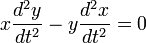 . .This is the resulting equation also in the derivation of the properties and the path of planetary motion from Newton's laws, which through integration and the introduction of polar coordinates, where ϑ is the angle between the radius vector and the positive abscissa and L is a constant, gives  . .We define the value  , ,Furthermore  and and  in the equations for  and and  then gives
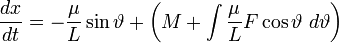
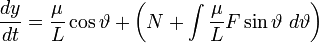
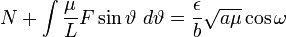
With the constants M and N through integration, this becomes
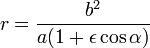
Because 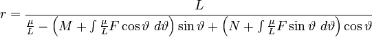 . .The integrals in the denominator gradually take other values, if F does not vanish. If we assume that we knew their value at a given time, then we could say that the planet is at this time on an ellipse described by these equations. If the semimajor axis is a, its semiminor axis b, the numerical eccentricity ε and the angle of a with the positive abscissae ω, then we solve the equations for  and 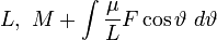 and and 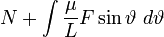 so we get
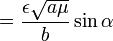
We see, by observing the immutability of  , ,and the other by  , ,dividing these gives
By equating the two expressions and with α=ϑ-ω we find that  , ,and working backwards gives 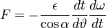 . .To gain an equation for
Thus 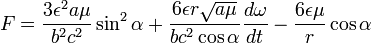 . .Therefore, the required equation for 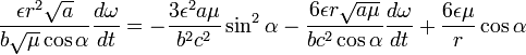 or after the definition of
If we want to compare the value of the velocity We multiply the equation for 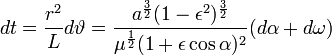 . .With suitable reordering and division, we get 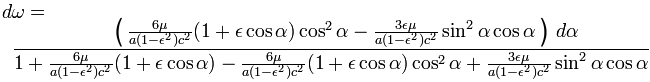 . .Dividing the numerator and denominator by 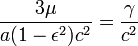 , ,we arrange in ascending powers of cos α, and use the abbreviation
so this becomes 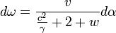 . .By approximating, we obtain ![d\omega=\left[\frac{v}{\frac{c^{2}}{\gamma}+2}-\frac{vw}{\left(\frac{c^{2}}{\gamma}+2\right)^{2}}\right]d\alpha](img/PG1-eqn77.png) . .For the perihelion movement ψ during an orbit, we therefore find ![\psi=\overset{2\pi}{\underset{0}{\int}}\left[\frac{v}{\frac{c^{2}}{\gamma}+2}-\frac{vw}{\left(\frac{c^{2}}{\gamma}+2\right)^{2}}\right]d\alpha](img/PG1-eqn78.png) or because
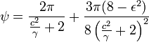 . .It follows that 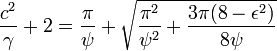 Considering that ψ is very small, we can see that the second term under the root vanishes against the first. The selected expression of approximation for dω is then still too precise, that is, w should have been discarded from the outset. This becomes
where for the same reason 2γ can be ignored compared with 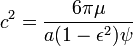 . .In this equation  , ,where τ is the orbital period of the planet. For Mercury in particular, the following values apply:
From this we find that The smallest speed of light found so far was by Foucault and was equal to 298000 km/sec; the largest comes from the method of Rømer with the latest observations of 308000 km/sec; in his experiments, Hertz found the speed of electrical waves to be 320000 km/sec. The speed of propagation of the gravitational potential is therefore consistent with the speed of light and electrical waves. This is at the same time the guarantee that this speed exists. Of course no one will deny that the perihelion movement of Mercury by 41" in a century could also be due to other, unknown factors, so that seeking a finite speed for gravitational potential might not be necessary. One has to remember, however, that the main deciding formula here, inducing moreover the deviation from all previous results of similar studies, for the dependence of the potential on such a completely natural speed, was progressively obtained without major assumptions. It would be a strange coincidence if the 41 arcseconds for Mercury equated precisely to the speed of light and electricity without having some connection with the spatial-temporal propagation of gravity, seeing that the medium in which this propagation and movement of light and electric waves happens, is the same as the space extending between the heavenly bodies. Not even the relatively large perihelion movement obtained with the values found for c for Venus, that is 8" in a century, can be considered a valid objection; or a review of the fluctuations of this planet would have to definitively exclude the possibility of that number. It is recalled that the calculations of the secular acceleration of the moon can fluctuate between 6" and 12". Moreover, there are nothing but imperceptibly small perihelion movements. They amount to the observed values easily found from the conventional tables of the earth in a century, 3.6", the moon 0.06", Mars 1.3", Jupiter 0.06", Saturn, 0.01", Uranus 0.002" and Neptune 0.0007". |
 ,
,
 ,
,
 .
. is small compared to c, we may substitute
  . This becomes
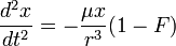 ,
,
 ,
, ,
,
 ,
, ,
,
 .
. , we find from the last two equations
 to
to ,
,
 ,
, .
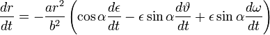
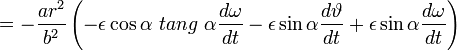
. , that the movement of the planet can be interpreted as if it was proceding along an ellipse whose ε and ω are changing constantly. This change only stops in the case that F = 0. It is thus through this change that the presence of a finite value of c comes into effect. We obtain for F, as soon as we differentiate the last two equations for θ, using the value of L and dividing the one by
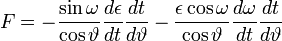 ,
,
 .
. contained in sizes observed in the middle of this value, we represent F by the derivatives of r by t. We have, again with allowance for the immutability of
  :
: ,
,
 ,
,


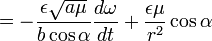 .
. and
and  and after division by

 and as long as the changes of ε against ε disappear themselves, we can view this as constant. It is sufficient then to choose as limits of integration a = 0 and a = 2π, since for each subsequent orbit
  ,
,
 ,
,
 ,
, ,
,
 ,
, . Finally we obtain